29.11 Visible and Ultra-Violet Spectroscopy (UV-Vis)

Visible and ultraviolet (UV-Vis spectroscopy) uses electromagnetic radiation to detect the presence of conjugated double bonds and can be used to quantify concentrations of a compound in a sample.

Conjugated Double Bonds

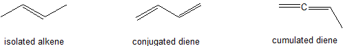
Conjugated dienes are characterized by alternating carbon-carbon double bonds separated by carbon-carbon single bonds. Cumulated dienes are characterized by adjacent carbon-carbon double bonds (Figure 29.11a.). While conjugated dienes are energetically more stable than isolated double bonds, cumulated double bonds are unstable.  Conjugated dienes are more stable than non-conjugated dienes (both isolated and cumulated) due to factors such as delocalization of charge through resonance and hybridization energy.

The Visible-Ultraviolet Spectrum

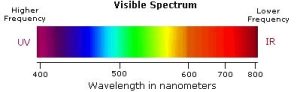
The visible spectrum constitutes but a small part of the total electromagnetic radiation spectrum (see Chapter 29.5 Spectroscopy Basics). Most of the radiation that surrounds us cannot be seen but can be detected by dedicated sensing instruments. The energy associated with a given segment of the spectrum is proportional to its frequency and inversely proportional to its wavelength (high wavelength = low frequency).  The visible portion of the spectrum is shown in Figure 29.11b.

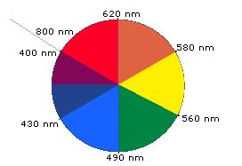
When white light passes through or is reflected by a coloured substance, a characteristic portion of the mixed wavelengths is absorbed. The remaining light will then assume the complementary colour to the wavelength(s) absorbed. This relationship is demonstrated by the colour wheel shown in Figure 29.11c. Here, complementary colours are diametrically opposite each other. Thus, absorption of 420-430 nm light renders a substance yellow, and absorption of 500-520 nm light makes it red. Green is unique in that it can be created by absorption close to 400 nm as well as absorption near 800 nm.

Early humans valued coloured pigments and used them for decorative purposes. Many of these were inorganic minerals, but several important organic dyes were also known. These included the crimson pigment, kermesic acid, the blue dye, indigo, and the yellow saffron pigment, crocetin. A rare dibromo-indigo derivative, punicin, was used to color the robes of the royal and wealthy. The deep orange hydrocarbon carotene is widely distributed in plants but is not sufficiently stable to be used as permanent pigment, other than for food colouring. A common feature of all these coloured compounds is a system of extensively conjugated π-electrons.

Transmittance and Absorbance

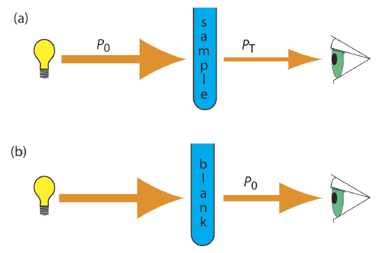
As light passes through a sample, its power decreases as some of it is absorbed. This attenuation of radiation is described quantitatively by two separate, but related terms: transmittance and absorbance. Transmittance is the ratio of the source radiation’s power as it exits the sample, P_T, to that incident on the sample, P₀ (Figure 29.11d.).  Multiplying the transmittance by 100 gives the percent transmittance, %T, which varies between 100% (no absorption) and 0% (complete absorption). All methods of detecting photons—including the human eye and modern photoelectric transducers—measure the transmittance of electromagnetic radiation.  In addition to absorption by the analyte, several additional phenomena contribute to the attenuation of radiation, including reflection and absorption by the sample’s container, absorption by other components in the sample’s matrix, and the scattering of radiation. To compensate for this loss of the radiation’s power, we use a method blank.

When monochromatic (single wavelength) electromagnetic radiation passes through a thin layer of sample of thickness, it experiences a decrease in its power.  This fractional decrease in power is proportional to the sample’s thickness and to the analyte’s concentration, C, in M or moles/L. The Beer-Lambert Law is:

A = εbC

where A is the absorbance, ε the molar absorptivity with units of cm^–1 M^–1 and b is the pathlength of the sample cell in cm.  The molar absorptivity is depended on the wavelength of the absorbed photon.  As such, there is a linear relationship between absorbance and concentration, resulting in calibration curves being used in quantitative analysis.

UV-Visible Absorption

To understand why some compounds are coloured and others are not, and to determine the relationship of conjugation to colour, we must make accurate measurements of light absorption at different wavelengths in and near the visible part of the spectrum. Commercial optical spectrometers enable such experiments to be conducted with ease, and usually survey both the near ultraviolet and visible portions of the spectrum.  The visible region of the spectrum comprises photon energies of 36 to 72 kcal/mole, and the near ultraviolet region, out to 200 nm, extends this energy range to 143 kcal/mole. Ultraviolet radiation having wavelengths less than 200 nm is difficult to handle and is seldom used as a routine tool for structural analysis.

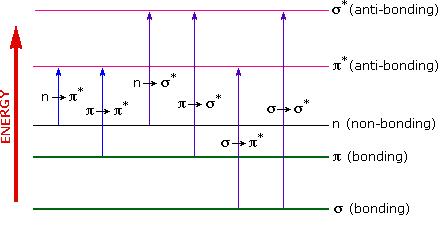
The energies in the visible and ultra-violet regions are sufficient to promote or excite a molecular electron to a higher energy orbital as seen in Figure 29.11e. Of the six transitions outlined, only the two lowest energy ones (left-most, coloured blue) are achieved by the energies available in the 200 to 800 nm spectrum. As a rule, energetically favoured electron promotion will be from the highest occupied molecular orbital (HOMO) to the lowest unoccupied molecular orbital (LUMO), and the resulting species is called an excited state.  Consequently, absorption spectroscopy carried out in this region is sometimes called “electronic spectroscopy”.

When sample molecules are exposed to light having an energy that matches a possible electronic transition within the molecule, some of the light energy will be absorbed as the electron is promoted to a higher energy orbital. An optical spectrometer records the wavelengths at which absorption occurs, together with the degree of absorption at each wavelength. The resulting spectrum is presented as a graph of absorbance (A) versus wavelength.  If a compound is colourless, it does not absorb in the visible part of the spectrum and this region is not displayed on the graph. Absorbance usually ranges from 0 (no absorption) to 2 (99% absorption) and is precisely defined in context with spectrometer operation.

Many electronic transitions of smaller molecules such as hydrogen or ethene are too energetic to be accurately recorded by standard UV spectrophotometers, which generally have a range of 220 – 700 nm. Where UV-vis spectroscopy becomes useful to most organic and biological chemists is in the study of molecules with conjugated pi systems. In these groups, the energy gap for π -π* transitions is smaller than for isolated double bonds, and thus the wavelength absorbed is longer. Molecules or parts of molecules that absorb light strongly in the UV-vis region are called chromophores.

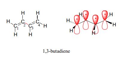
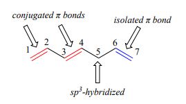
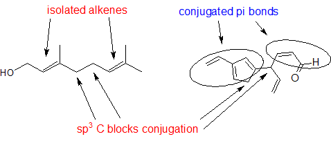
1,3-butadiene (Figure 29.11f.) is the simplest example of a system of conjugated pi bonds. To be considered conjugated, two or more pi bonds must be separated by only one single bond – in other words, there cannot be an intervening sp³-hybridized carbon, because this would break up the overlapping system of parallel p orbitals. In Figure 29.11g., the compound’s C₁-C₂ and C₃-C₄ double bonds are conjugated, while the C₆-C₇ double bond is isolated from the other two pi bonds by sp³-hybridized C₅.

 

 

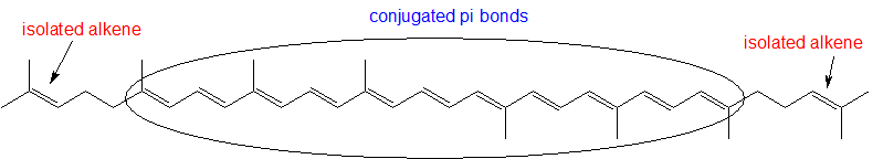
Conjugated pi systems can involve oxygen and nitrogen atoms as well as carbon. In the metabolism of fat molecules, some of the key reactions involve alkenes that are conjugated to carbonyl groups.  In molecules with extended pi systems, the HOMO-LUMO energy gap becomes so small that absorption occurs in the visible rather than the UV region of the electromagnetic spectrum. Beta-carotene (Figure 29.11h.), with its system of 11 conjugated double bonds, absorbs light with wavelengths in the blue region of the visible spectrum while allowing other visible wavelengths – mainly those in the red-yellow region – to be transmitted. This is why carrots are orange.

Example 29.11a

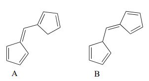
Identify all conjugated and isolated double bonds in the structures below.

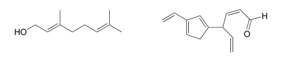
Solution:

Look for sp³ hybridized carbons to find disruptions in conjugation.

 

Source: Exercise adapted from Map: Organic Chemistry (Wade), CC BY-NC-SA 4.0.

Exercise 29.11a

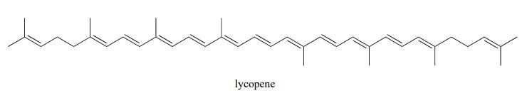
Identify all isolated and conjugated pi bonds in lycopene, the red-coloured compound in tomatoes.

Check Your Answer:^[1]

Source: Exercise and images in solution adapted from Map: Organic Chemistry (Wade), CC BY-NC-SA 4.0.

UV-Vis Spectra

The basic setup for a UV-vis absorbance spectrophotometer is the same as for IR spectroscopy: radiation with a range of wavelengths is directed through a sample of interest, and a detector records which wavelengths were absorbed and to what extent the absorption occurred.

Figure 29.11l. is the absorbance spectrum of an important biological molecule called nicotinamide adenine dinucleotide, abbreviated NAD^{+ .} This compound absorbs light in the UV range due to the presence of conjugated pi-bonding systems.

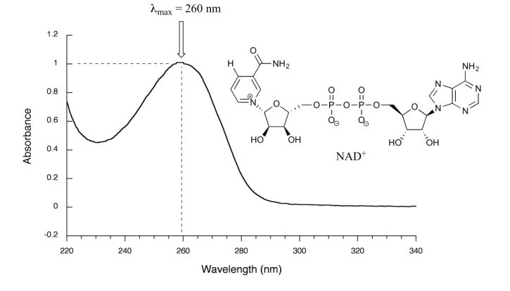
This UV spectrum is much simpler than the IR spectra seen in previous sections: this one has only one peak, although many molecules have more than one. Notice also that the convention in UV-Vis spectroscopy is to show the baseline at the bottom of the graph with the peaks pointing up. Wavelength values on the x-axis are generally measured in nanometers (nm) rather than in cm^-1 as is the convention in IR spectroscopy.

Peaks in UV spectra tend to be quite broad, often spanning well over 20 nm at half-maximal height. Typically, there are two things that are looked for and record from a UV-Vis spectrum. The first is λ_max, which is the wavelength at maximal light absorbance. For NAD⁺, its λ_max, = 260 nm. Second is how much light is absorbed at λ_max, called absorbance, abbreviated ‘A’ with no units. This contains the same information as the ‘percent transmittance’ number used in IR spectroscopy, just expressed in slightly different terms. To calculate absorbance at a given wavelength, the computer in the spectrophotometer simply takes the intensity of light at that wavelength before it passes through the sample (I₀), divides this value by the intensity of the same wavelength after it passes through the sample (I), then takes the log₁₀ of that number: A = log I₀/I.

Figure 29.11m. shows the absorbance spectrum of the common food colouring Red #3. Here, the extended system of conjugated pi bonds causes the molecule to absorb light in the visible range. Because the λ_max of 524 nm falls within the green region of the spectrum, the compound appears red to our eyes.

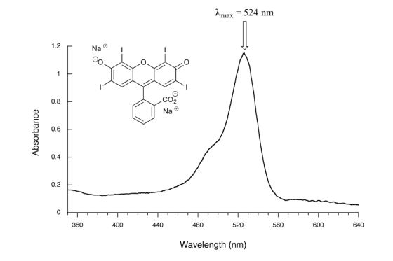
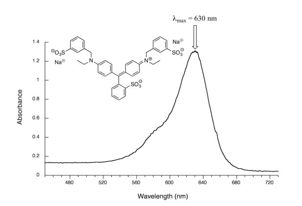
Figure 29.11n. is the spectrum of another food colouring, Blue #1. Here, maximum absorbance is at 630 nm, in the orange range of the visible spectrum, and the compound appears blue.

Exercise 29.11b

Which of the following molecules would you expect absorb at a longer wavelength in the UV region of the electromagnetic spectrum? Explain your answer.

Check Your Answer: ^[2]

Source: Exercise adapted from Organic Chem: Biological Emphasis Vol I (page 222), CC BY-NC-SA 4.0.

Watch Conjugation & UV-Vis Spectroscopy: Crash Course Organic Chemistry #41 – YouTube (13 min).

Quantitative Applications

The determination of an analyte’s concentration based on its absorption of ultraviolet or visible radiation is one of the most frequently encountered quantitative analytical methods. One reason for its popularity is that many organic and inorganic compounds have strong absorption bands in the UV/Vis region of the electromagnetic spectrum. In addition, if an analyte does not absorb UV/Vis radiation—or if its absorbance is too weak— it often can be reacted with another species that is strongly absorbing. For example, a dilute solution of Fe²⁺ does not absorb visible light. Reacting Fe²⁺ with o-phenanthroline, however, forms an orange–red complex of Fe(phen)₃²⁺ that has a strong, broad absorbance band near 500 nm. An additional advantage to UV/Vis absorption is that in most cases it is relatively easy to adjust experimental and instrumental conditions so that Beer’s law is obeyed.

The analysis of waters and wastewaters often relies on the absorption of ultraviolet and visible radiation.  Aluminum, arsenic, cadmium, chromium, copper, iron, lead, manganese, mercury, zinc, ammonia, cyanide, fluoride, chlorine, nitrate, nitrate, phosphate and many more can be measured using UV-Vis spectroscopy.  Refer to the procedure manual of your model of spectrophotometer.  For example, this site lists the Methods/Procedures for the HACH DR3900 Laboratory VIS Spectrophotometer.

Spotlight on Everyday Chemistry: Drinking Water Disinfection

Chlorine is used to disinfect and treat most drinking water at water treatment plants throughout Canada. This is used to treat the water at the source/treatment plant as well as maintain a chlorine residual in the distribution system to prevent bacterial growth.  When chlorine is added to water the portion available for disinfection is called the chlorine residual (Government of Canada, 2016, para. 2).

There are two forms of chlorine residual. The free chlorine residual includes Cl₂, HOCl, and OCl^–. The combined chlorine residual, which forms from the reaction of NH₃ with HOCl, consists of monochloramine, NH₂Cl, dichloramine, NHCl₂, and trichloramine, NCl₃. Because the free chlorine residual is more efficient as a disinfectant, there is an interest in methods that can distinguish between the total chlorine residual’s different forms.

One such method is the leuco crystal violet method. The free residual chlorine is determined by adding leuco crystal violet to the sample, which instantaneously oxidizes to give a blue-coloured compound that is monitored at 592 nm. Completing the analysis in less than five minutes prevents a possible interference from the combined chlorine residual. The total chlorine residual (free + combined) is determined by reacting a separate sample with iodide, which reacts with both chlorine residuals to form HOI. When the reaction is complete, leuco crystal violet is added and oxidized by HOI, giving the same blue-coloured product. The combined chlorine residual is determined by difference.

Read more about the disinfection of drinking water in Ontario at Ontario.ca and the Guidelines for Canadian Drinking Water Quality: Guideline Technical Document – Chlorine – Canada.ca

Source: Instrumental Analysis, CC BY-NC-SA 4.0

Example 29.11b

The determination of iron in an industrial waste stream is carried out by the o-phenanthroline method. Using the data in the following table, determine the mg Fe/L in the waste stream.

mg Fe/L	absorbance
0.00	0.000
1.00	0.183
2.00	0.364
3.00	0.546
4.00	0.727
sample	0.269

Solution:

Linear regression (using a spreadsheet) of absorbance versus the concentration of Fe in the standards gives the calibration curve and calibration equation shown.

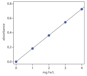
A=0.0006 + (0.1817 mg−1 L) × (mg Fe/L)

$$$$

Substituting the sample’s absorbance into the calibration equation gives the concentration of Fe in the waste stream as 1.48 mg Fe/L.  Alternatively, the curve can be used to estimate about 1.5 mg Fe/L.

Source: Example adapted from Credit: Instrumental Analysis, CC BY-NC-SA 4.0.

Attribution & References

Except where otherwise noted, this page is adapted by Samantha Sullivan Sauer from

• “13.1: Transmittance and Absorbance“, “13.2: Beer’s Law“, “14.4: Quantitative Applications” by David Harvey In Instrumental Analysis, licensed under a CC BY-NC-SA 4.0
• “16.1: Stability of Conjugated Dienes – Molecular Orbital Theory”  In Map: Organic Chemistry (Wade), Complete and Semesters I and II by LibreTexts, licensed under CC BY-NC-SA 4.0. Contributors from original source:
  • Dr. Dietmar Kennepohl FCIC (Professor of Chemistry, Athabasca University)
  • Prof. Steven Farmer (Sonoma State University)
  • William Reusch, Professor Emeritus (Michigan State U.), Virtual Textbook of Organic Chemistry
  • Organic Chemistry With a Biological Emphasis by Tim Soderberg (University of Minnesota, Morris)
• “16.10: Interpreting Ultraviolet Spectra – The Effect of Conjugation” In Map: Organic Chemistry (Wade), Complete and Semesters I and II by LibreTexts, licensed under CC BY-NC-SA 4.0. Contributors from original source:
  • Dr. Dietmar Kennepohl FCIC (Professor of Chemistry, Athabasca University),
  • Prof. Steven Farmer (Sonoma State University),
  • William Reusch, Professor Emeritus (Michigan State U.),
  • Virtual Textbook of Organic Chemistry, Organic Chemistry With a Biological Emphasis by Tim Soderberg (University of Minnesota, Morris)
• “16.9: Structure Determination in Conjugated Systems – Ultraviolet Spectroscopy”  In Map: Organic Chemistry (Wade), Complete and Semesters I and IIby LibreTexts, licensed under CC BY-NC-SA 4.0. Contributors from original source:
  • Prof. Steven Farmer (Sonoma State University)
  • Organic Chemistry With a Biological Emphasis by Tim Soderberg (University of Minnesota, Morris)

References cited in text