10.3 Wave Nature of Matter

Wave Behaviour of Matter from a Microscopic Perspective

We know how matter behaves in the macroscopic world – objects that are large enough to be seen by the naked eye follow the rules of classical physics. A billiard ball moving on a table will behave like a particle: It will continue in a straight line unless it collides with another ball or the table cushion, or is acted on by some other force (such as friction). The ball has a well-defined position and velocity (or a well-defined momentum, p = mv, defined by mass m and velocity v) at any given moment. In other words, the ball is moving in a classical trajectory. This is the typical behaviour of a classical object.

When waves interact with each other, they show interference patterns that are not displayed by macroscopic particles such as the billiard ball. For example, interacting waves on the surface of water can produce interference patterns similar to those shown on Figure 10.3a. This is a case of wave behaviour on the macroscopic scale, and it is clear that particles and waves are very different phenomena in the macroscopic realm.

As technological improvements allowed scientists to probe the microscopic world in greater detail, it became increasingly clear by the 1920s that very small pieces of matter follow a different set of rules from those we observe for large objects. The unquestionable separation of waves and particles was no longer the case for the microscopic world.

One of the first people to pay attention to the special behaviour of the microscopic world was Louis de Broglie. He asked the question: If electromagnetic radiation can have particle-like character, can electrons and other submicroscopic particles exhibit wavelike character? In his 1925 doctoral dissertation, de Broglie extended the wave–particle duality of light that Einstein used to resolve the photoelectric-effect paradox to material particles. He predicted that a particle with mass m and velocity v (that is, with linear momentum p) should also exhibit the behaviour of a wave with a wavelength value λ, given by this expression in which h is the familiar Planck’s constant:

This is called the de Broglie wavelength. Unlike the other values of λ discussed in this chapter, the de Broglie wavelength is a characteristic of particles and other bodies, not electromagnetic radiation (note that this equation involves velocity [v, m/s], not frequency [ν, Hz]. Although these two symbols are identical, they mean very different things). Where Bohr had postulated the electron as being a particle orbiting the nucleus in quantized orbits, de Broglie argued that Bohr’s assumption of quantization can be explained if the electron is considered not as a particle, but rather as a circular standing wave such that only an integer number of wavelengths could fit exactly within the orbit (Figure 10.3b).

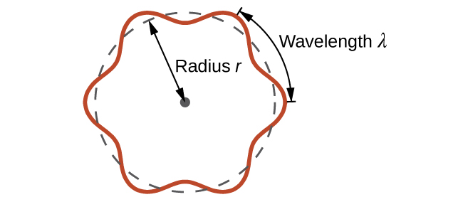
For a circular orbit of radius r, the circumference is 2πr, and so de Broglie’s condition is:

Since the de Broglie expression relates the wavelength to the momentum and, hence, velocity, this implies:

This expression can be rearranged to give Bohr’s formula for the quantization of the angular momentum:

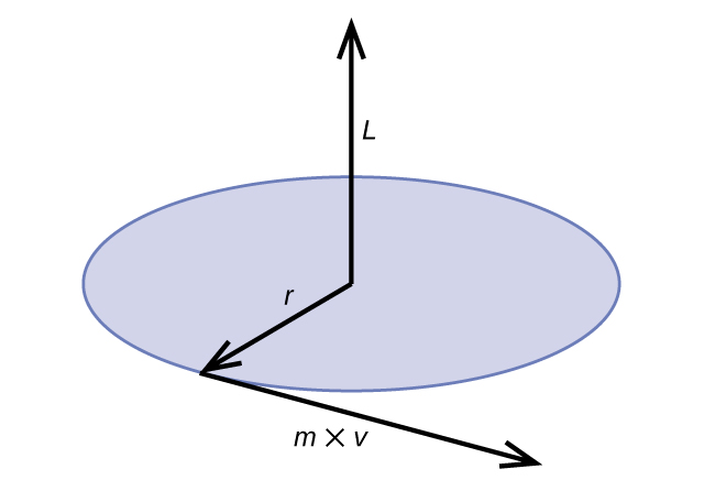
Classical angular momentum L for a circular motion is equal to the product of the radius of the circle and the momentum of the moving particle p (Figure 10.3c).

Shortly after de Broglie proposed the wave nature of matter, two scientists at Bell Laboratories, C. J. Davisson and L. H. Germer, demonstrated experimentally that electrons can exhibit wavelike behaviour by showing an interference pattern for electrons travelling through a regular atomic pattern in a crystal. The regularly spaced atomic layers served as slits, as used in other interference experiments. Since the spacing between the layers serving as slits needs to be similar in size to the wavelength of the tested wave for an interference pattern to form, Davisson and Germer used a crystalline nickel target for their “slits,” since the spacing of the atoms within the lattice was approximately the same as the de Broglie wavelengths of the electrons that they used. Figure 10.3d shows an interference pattern.

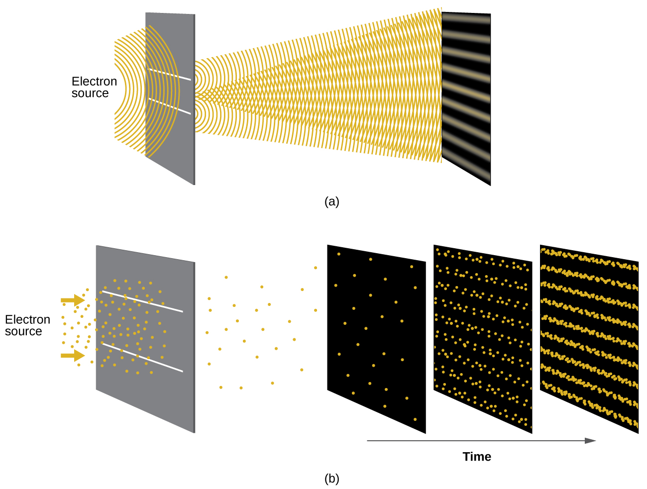
The wave–particle duality of matter can be seen in Figure 10.3d by observing what happens if electron collisions are recorded over a long period of time. Initially, when only a few electrons have been recorded, they show clear particle-like behaviour, having arrived in small localized packets that appear to be random. As more and more electrons arrived and were recorded, a clear interference pattern that is the hallmark of wavelike behaviour emerged. Thus, it appears that while electrons are small localized particles, their motion does not follow the equations of motion implied by classical mechanics, but instead it is governed by some type of a wave equation that governs a probability distribution even for a single electron’s motion. Thus the wave–particle duality first observed with photons is actually a fundamental behaviour intrinsic to all quantum particles.

Watch Dr. Quantum – Double Slit Experiment (5min 12s)

We never think of a thrown softball having a wavelength, since this wavelength is so small it is impossible for our senses or any known instrument to detect (strictly speaking, the wavelength of a real baseball would correspond to the wavelengths of its constituent atoms and molecules, which, while much larger than this value, would still be microscopically tiny). The de Broglie wavelength is only appreciable for matter that has a very small mass and/or a very high velocity.

Werner Heisenberg considered the limits of how accurately we can measure properties of an electron or other microscopic particles. He determined that there is a fundamental limit to how accurately one can measure both a particle’s position and its momentum simultaneously. The more accurately we measure the momentum of a particle, the less accurately we can determine its position at that time, and vice versa. This is summed up in what we now call the Heisenberg uncertainty principle: It is fundamentally impossible to determine simultaneously and exactly both the momentum and the position of a particle. For a particle of mass m moving with velocity v_x in the x direction (or equivalently with momentum p_x), the product of the uncertainty in the position, Δx, and the uncertainty in the momentum, Δp_x , must be greater than or equal to [latex]\frac{\hbar}{2}[/latex] (recall that [latex]\hbar = \frac{h}{2 \pi}[/latex], the value of Planck’s constant divided by 2π).

This equation allows us to calculate the limit to how precisely we can know both the simultaneous position of an object and its momentum. For example, if we improve our measurement of an electron’s position so that the uncertainty in the position (Δx) has a value of, say, 1 pm (10^–12 m, about 1% of the diameter of a hydrogen atom), then our determination of its momentum must have an uncertainty with a value of at least