14.2 Solubility
Learning Objectives
- Describe the effects of temperature and pressure on solubility
- State Henry’s law and use it in calculations involving the solubility of a gas in a liquid
- Explain the degrees of solubility possible for liquid-liquid solutions
Imagine adding a small amount of salt to a glass of water, stirring until all the salt has dissolved, and then adding a bit more. You can repeat this process until the salt concentration of the solution reaches its natural limit, a limit determined primarily by the relative strengths of the solute-solute, solute-solvent, and solvent-solvent attractive forces discussed in the previous module of this chapter. You can be certain that you have reached this limit because, no matter how long you stir the solution, undissolved salt remains. The concentration of salt in the solution at this point is known as its solubility.
The solubility of a solute in a particular solvent is the maximum concentration that may be achieved under given conditions when the dissolution process is at equilibrium. Referring to the example of salt in water:
When a solute’s concentration is equal to its solubility, the solution is said to be saturated with that solute. If the solute’s concentration is less than its solubility, the solution is said to be unsaturated. A solution that contains a relatively low concentration of solute is called dilute, and one with a relatively high concentration is called concentrated.
If we add more salt to a saturated solution of salt, we see it fall to the bottom and no more seems to dissolve. In fact, the added salt does dissolve, as represented by the forward direction of the dissolution equation. Accompanying this process, dissolved salt will precipitate, as depicted by the reverse direction of the equation. The system is said to be at equilibrium when these two reciprocal processes are occurring at equal rates, and so the amount of undissolved and dissolved salt remains constant. Support for the simultaneous occurrence of the dissolution and precipitation processes is provided by noting that the number and sizes of the undissolved salt crystals will change over time, though their combined mass will remain the same.
Exercise 14.2a
Practice using the following PhET simulation: Salts & Solubility
Solutions in which a solute concentration exceeds its solubility may be prepared. Such solutions are said to be supersaturated, and they are interesting examples of nonequilibrium states. For example, the carbonated beverage in an open container that has not yet “gone flat” is supersaturated with carbon dioxide gas; given time, the CO2 concentration will decrease until it reaches its equilibrium value.
Watch Crystal Growing – Cool Science Experiment (3 mins)
Video source: Sick Science! (2009, December 15). Crystal Growing – Cool Science Experiment [Video]. YouTube.
Watch crystallization of sodium acetate (v2) (2 min)
Video source: BerkeleyChemDemos. (2013, October 10). Crystallization of sodium acetate (v2) [Video]. YouTube.
Solutions of Gases in Liquids
In an earlier module of this chapter, the effect of intermolecular attractive forces on solution formation was discussed. The chemical structures of the solute and solvent dictate the types of forces possible and, consequently, are important factors in determining solubility. For example, under similar conditions, the water solubility of oxygen is approximately three times greater than that of helium, but 100 times less than the solubility of chloromethane, CHCl3. Considering the role of the solvent’s chemical structure, note that the solubility of oxygen in the liquid hydrocarbon hexane, C6H14, is approximately 20 times greater than it is in water.
Other factors also affect the solubility of a given substance in a given solvent. Temperature is one such factor, with gas solubility typically decreasing as temperature increases (Figure 14.2a). This is one of the major impacts resulting from the thermal pollution of natural bodies of water.

When the temperature of a river, lake, or stream is raised abnormally high, usually due to the discharge of hot water from some industrial process, the solubility of oxygen in the water is decreased. Decreased levels of dissolved oxygen may have serious consequences for the health of the water’s ecosystems and, in severe cases, can result in large-scale fish kills (Figure 14.2b).
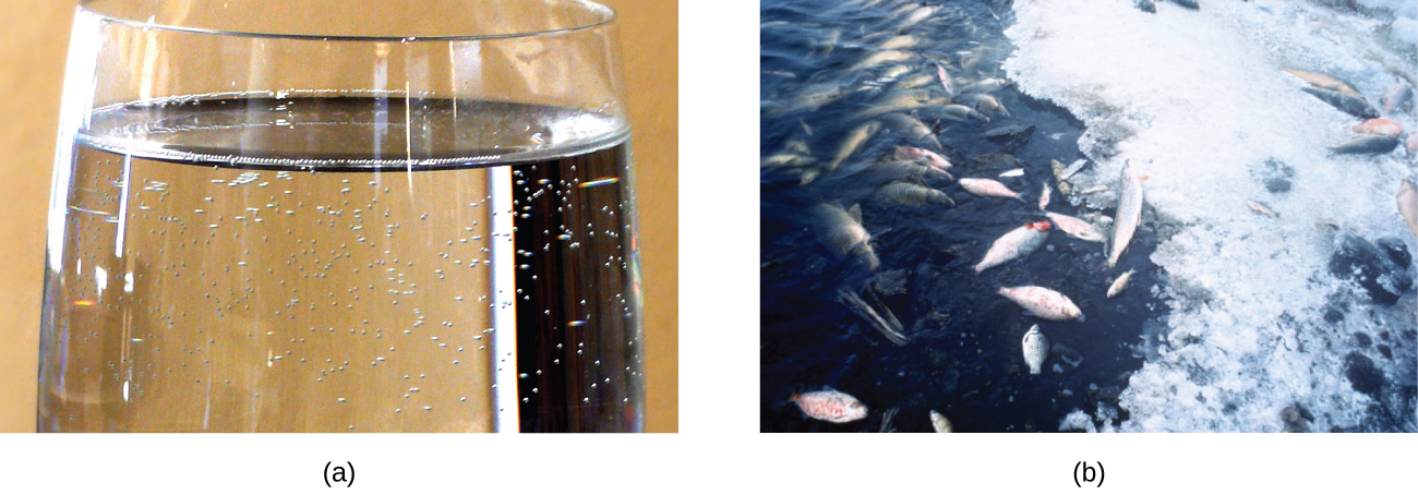
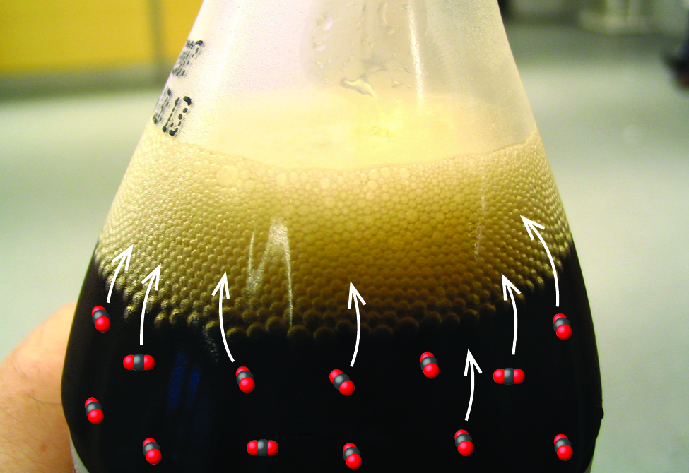
The solubility of a gaseous solute is also affected by the partial pressure of solute in the gas to which the solution is exposed. Gas solubility increases as the pressure of the gas increases. Carbonated beverages provide a nice illustration of this relationship. The carbonation process involves exposing the beverage to a relatively high pressure of carbon dioxide gas and then sealing the beverage container, thus saturating the beverage with CO2 at this pressure. When the beverage container is opened, a familiar hiss is heard as the carbon dioxide gas pressure is released, and some of the dissolved carbon dioxide is typically seen leaving solution in the form of small bubbles (Figure 14.2c). At this point, the beverage is supersaturated with carbon dioxide and, with time, the dissolved carbon dioxide concentration will decrease to its equilibrium value and the beverage will become “flat.”
For many gaseous solutes, the relationship between solubility, Cg, and partial pressure, Pg, is a proportional one:
where k is a proportionality constant that depends on the identities of the gaseous solute and solvent, and on the solution temperature. This is a mathematical statement of Henry’s law: The quantity of an ideal gas that dissolves in a definite volume of liquid is directly proportional to the pressure of the gas.
Example 14.2a
Application of Henry’s Law
At 20 °C, the concentration of dissolved oxygen in water exposed to gaseous oxygen at a partial pressure of 101.3 kPa (760 torr) is 1.38 × 10⁻³ mol L−1. Use Henry’s law to determine the solubility of oxygen when its partial pressure is 20.7 kPa (155 torr), the approximate pressure of oxygen in earth’s atmosphere.
Solution
According to Henry’s law, for an ideal solution the solubility, Cg, of a gas (1.38 × 10⁻³ mol L−1, in this case) is directly proportional to the pressure, Pg, of the undissolved gas above the solution (101.3 kPa, or 760 torr, in this case). Because we know both Cg and Pg, we can rearrange this expression to solve for k.
Now we can use k to find the solubility at the lower pressure.
Note that various units may be used to express the quantities involved in these sorts of computations. Any combination of units that yield to the constraints of dimensional analysis are acceptable.
Exercise 14.2b
Exposing a 100.0 mL sample of water at 0 °C to an atmosphere containing a gaseous solute at 20.26 kPa (152 torr) resulted in the dissolution of 1.45 × 10⁻³ g of the solute. Use Henry’s law to determine the solubility of this gaseous solute when its pressure is 101.3 kPa (760 torr).
Check Your Answer[1]
Decompression Sickness or “The Bends”
Decompression sickness (DCS), or “the bends,” is an effect of the increased pressure of the air inhaled by scuba divers when swimming underwater at considerable depths. In addition to the pressure exerted by the atmosphere, divers are subjected to additional pressure due to the water above them, experiencing an increase of approximately 1 atm for each 10 m of depth. Therefore, the air inhaled by a diver while submerged contains gases at the corresponding higher ambient pressure, and the concentrations of the gases dissolved in the diver’s blood are proportionally higher per Henry’s law.
As the diver ascends to the surface of the water, the ambient pressure decreases and the dissolved gases becomes less soluble. If the ascent is too rapid, the gases escaping from the diver’s blood may form bubbles that can cause a variety of symptoms ranging from rashes and joint pain to paralysis and death. To avoid DCS, divers must ascend from depths at relatively slow speeds (10 or 20 m/min) or otherwise make several decompression stops, pausing for several minutes at given depths during the ascent. When these preventive measures are unsuccessful, divers with DCS are often provided hyperbaric oxygen therapy in pressurized vessels called decompression (or recompression) chambers (Figure 14.2d).
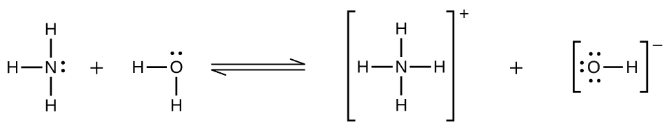
Deviations from Henry’s law are observed when a chemical reaction takes place between the gaseous solute and the solvent. Thus, for example, the solubility of ammonia in water does not increase as rapidly with increasing pressure as predicted by the law because ammonia, being a base, reacts to some extent with water to form ammonium ions and hydroxide ions.
Solutions of Liquids in Liquids
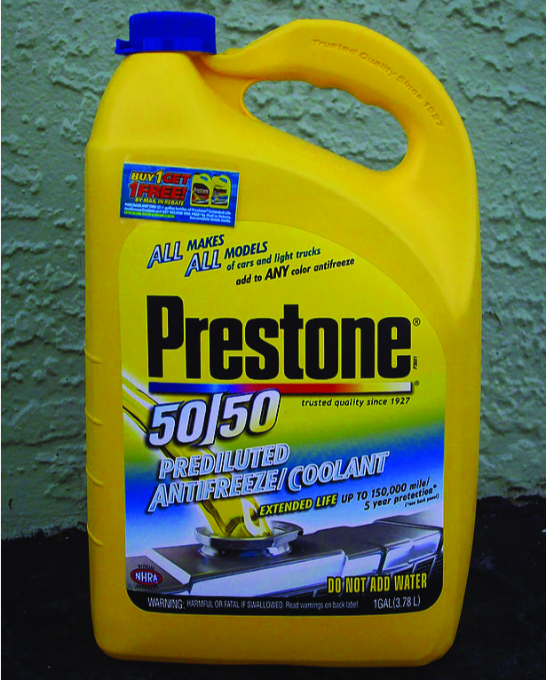
We know that some liquids mix with each other in all proportions; in other words, they have infinite mutual solubility and are said to be miscible. Ethanol, sulfuric acid, and ethylene glycol (popular for use as antifreeze, pictured in Figure 14.2e) are examples of liquids that are completely miscible with water. Two-cycle motor oil is miscible with gasoline.
Liquids that mix with water in all proportions are usually polar substances or substances that form hydrogen bonds. For such liquids, the dipole-dipole attractions (or hydrogen bonding) of the solute molecules with the solvent molecules are at least as strong as those between molecules in the pure solute or in the pure solvent. Hence, the two kinds of molecules mix easily. Likewise, nonpolar liquids are miscible with each other because there is no appreciable difference in the strengths of solute-solute, solvent-solvent, and solute-solvent intermolecular attractions. The solubility of polar molecules in polar solvents and of nonpolar molecules in nonpolar solvents is, again, an illustration of the chemical axiom “like dissolves like.”
Two liquids that do not mix to an appreciable extent are called immiscible. Layers are formed when we pour immiscible liquids into the same container. Gasoline, oil (Figure 14.2f), benzene, carbon tetrachloride, some paints, and many other nonpolar liquids are immiscible with water. The attraction between the molecules of such nonpolar liquids and polar water molecules is ineffectively weak. The only strong attractions in such a mixture are between the water molecules, so they effectively squeeze out the molecules of the nonpolar liquid. The distinction between immiscibility and miscibility is really one of degrees, so that miscible liquids are of infinite mutual solubility, while liquids said to be immiscible are of very low (though not zero) mutual solubility.
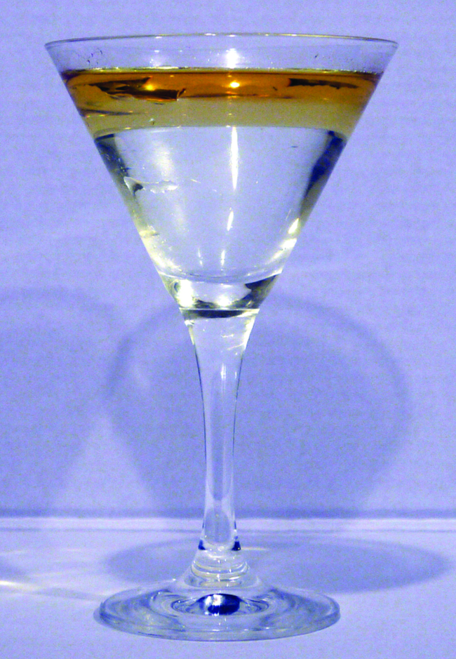
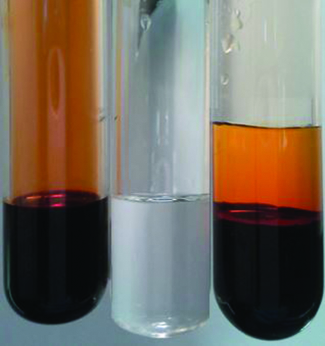
Two liquids, such as bromine and water, that are of moderate mutual solubility are said to be partially miscible. Two partially miscible liquids usually form two layers when mixed. In the case of the bromine and water mixture, the upper layer is water, saturated with bromine, and the lower layer is bromine saturated with water. Since bromine is nonpolar, and, thus, not very soluble in water, the water layer is only slightly discoloured by the bright orange bromine dissolved in it. Since the solubility of water in bromine is very low, there is no noticeable effect on the dark colour of the bromine layer (Figure 14.2g).
Solutions of Solids in Liquids
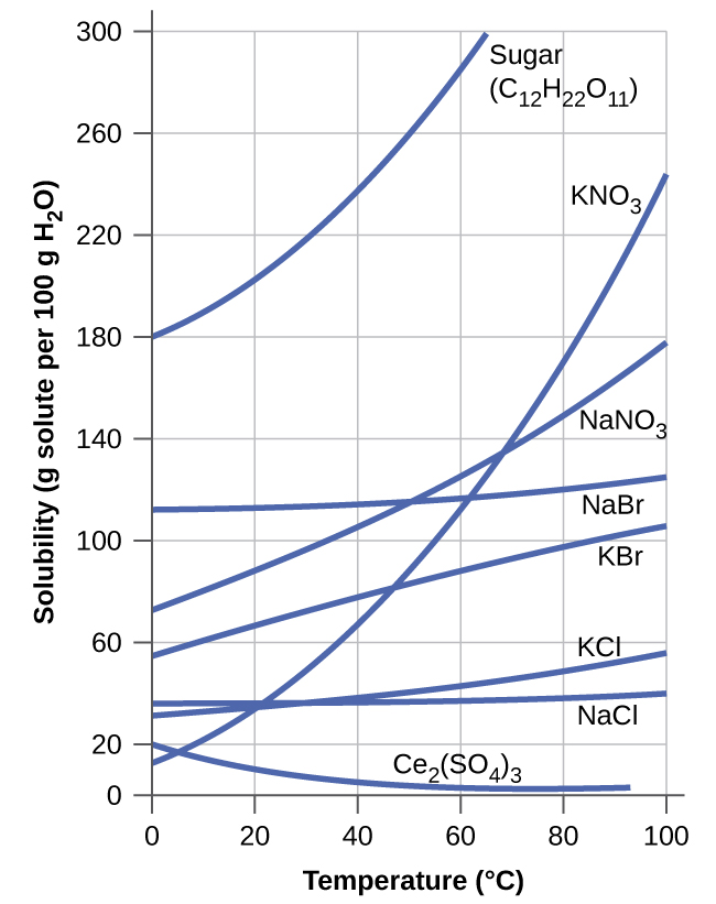
The dependence of solubility on temperature for a number of inorganic solids in water is shown by the solubility curves in Figure 14.2h. Reviewing these data indicate a general trend of increasing solubility with temperature, although there are exceptions, as illustrated by the ionic compound cerium sulfate.
The temperature dependence of solubility can be exploited to prepare supersaturated solutions of certain compounds. A solution may be saturated with the compound at an elevated temperature (where the solute is more soluble) and subsequently cooled to a lower temperature without precipitating the solute. The resultant solution contains solute at a concentration greater than its equilibrium solubility at the lower temperature (i.e., it is supersaturated) and is relatively stable. Precipitation of the excess solute can be initiated by adding a seed crystal (see the video in the Link to Learning earlier in this module) or by mechanically agitating the solution. Some hand warmers take advantage of this behaviour.
Watch Crystallization of the “Magic” Gel Hand Warmer bag (HD) (1 min)
Video source: Filipe Rodrigues. (2014, January 4). Crystallization of the “Magic” Gel Hand Warmer bag (HD) [Video]. YouTube.
Solubility of Ionic Compounds
The solubility of ionic compounds can be predicted based on the nature of the cations and anions present in the compound. Compounds that are soluble (along with their exceptions) can be seen in Table 14.2a, while those that are insoluble (along with their exceptions) can be seen in Table 14.2b.
Source: “Table 14.2a” by Gregory Anderson is adapted from “4.2 Classifying Chemical Reactions” in Chemistry (OpenStax), CC BY 4.0
Source: “Table 14.2b” by Gregory Anderson is adapted from “4.2 Classifying Chemical Reactions” in Chemistry (OpenStax), CC BY 4.0
Links to Interactive Learning Tools
Explore Precipitation Reactions from the Physics Classroom.
Practice Solution Word Definitions from eCampusOntario H5P Studio.
Key Equations
- [latex]C_{\text{g}} = kP_{\text{g}}[/latex]
Attribution & References
- 7.25 × 10⁻³ in 100.0 mL or 0.0725 g/L ↵
extent to which a solute may be dissolved in water, or any solvent
of concentration equal to solubility; containing the maximum concentration of solute possible for a given temperature and pressure
of concentration less than solubility
of concentration that exceeds solubility; a nonequilibrium state
law stating the proportional relationship between the concentration of dissolved gas in a solution and the partial pressure of the gas in contact with the solution
mutually soluble in all proportions; typically refers to liquid substances
of negligible mutual solubility; typically refers to liquid substances
of moderate mutual solubility; typically refers to liquid substances
