12.5 The Kinetic-Molecular Theory

The Kinetic-Molecular Theory Explains the Behaviour of Gases, Part I

Recalling that gas pressure is exerted by rapidly moving gas molecules and depends directly on the number of molecules hitting a unit area of the wall per unit of time, we see that the KMT conceptually explains the behaviour of a gas as follows:

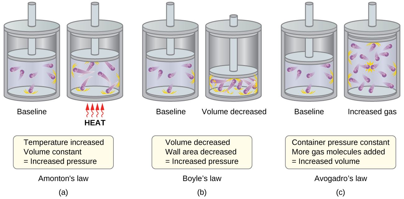
• Amonton’s / Gay-Lussac’s law: If the temperature is increased, the average speed and kinetic energy of the gas molecules increase. If the volume is held constant, the increased speed of the gas molecules results in more frequent and more forceful collisions with the walls of the container, therefore increasing the pressure (Figure 12.5a.a).
• Charles’ law: If the temperature of a gas is increased, a constant pressure may be maintained only if the volume occupied by the gas increases. This will result in greater average distances traveled by the molecules to reach the container walls, as well as increased wall surface area. These conditions will decrease both the frequency of molecule-wall collisions and the number of collisions per unit area, the combined effects of which balance the effect of increased collision forces due to the greater kinetic energy at the higher temperature.
• Boyle’s law: If the gas volume is decreased, the container wall area decreases and the molecule-wall collision frequency increases, both of which increase the pressure exerted by the gas (Figure 12.5a.b).
• Avogadro’s law: At constant pressure and temperature, the frequency and force of molecule-wall collisions are constant. Under such conditions, increasing the number of gaseous molecules will require a proportional increase in the container volume in order to yield a decrease in the number of collisions per unit area to compensate for the increased frequency of collisions (Figure 12.5a.c).
• Dalton’s Law: Because of the large distances between them, the molecules of one gas in a mixture bombard the container walls with the same frequency whether other gases are present or not, and the total pressure of a gas mixture equals the sum of the (partial) pressures of the individual gases.

Molecular Velocities and Kinetic Energy

The previous discussion showed that the KMT qualitatively explains the behaviours described by the various gas laws. The postulates of this theory may be applied in a more quantitative fashion to derive these individual laws. To do this, we must first look at velocities and kinetic energies of gas molecules, and the temperature of a gas sample.

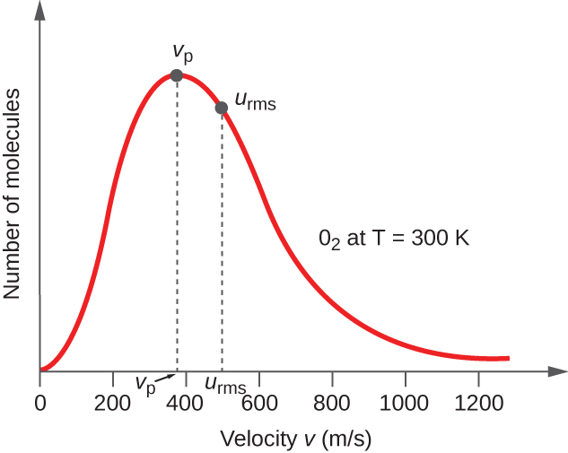
In a gas sample, individual molecules have widely varying speeds; however, because of the vast number of molecules and collisions involved, the molecular speed distribution and average speed are constant. This molecular speed distribution is known as a Maxwell-Boltzmann distribution, and it depicts the relative numbers of molecules in a bulk sample of gas that possesses a given speed (Figure 12.5b).

The kinetic energy (KE) of a particle of mass (m) and speed (u) is given by:

Expressing mass in kilograms and speed in meters per second will yield energy values in units of joules (J = kg m² s^–2). To deal with a large number of gas molecules, we use averages for both speed and kinetic energy. In the KMT, the root mean square velocity of a particle, u_rms, is defined as the square root of the average of the squares of the velocities with n = the number of particles:

The average kinetic energy, KE_avg, is then equal to:

The KE_avg of a collection of gas molecules is also directly proportional to the temperature of the gas and may be described by the equation:

where R is the gas constant and T is the kelvin temperature. When used in this equation, the appropriate form of the gas constant is 8.314 J/K (8.314 kg m²s^–2K^–1). These two separate equations for KE_avg may be combined and rearranged to yield a relation between molecular speed and temperature:

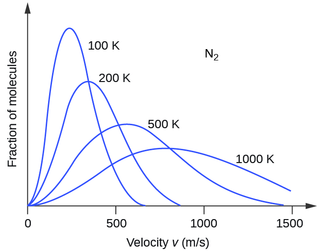
If the temperature of a gas increases, its KE_avg increases, more molecules have higher speeds and fewer molecules have lower speeds, and the distribution shifts toward higher speeds overall, that is, to the right. If temperature decreases, KE_avg decreases, more molecules have lower speeds and fewer molecules have higher speeds, and the distribution shifts toward lower speeds overall, that is, to the left. This behaviour is illustrated for nitrogen gas in Figure 12.5c.

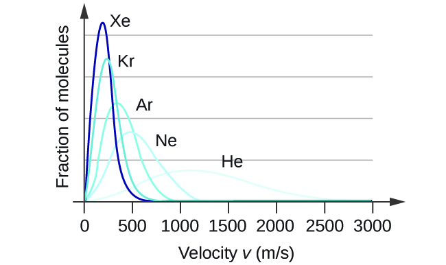
At a given temperature, all gases have the same KE_avg for their molecules. Gases composed of lighter molecules have more high-speed particles and a higher u_rms, with a speed distribution that peaks at relatively higher velocities. Gases consisting of heavier molecules have more low-speed particles, a lower u_rms, and a speed distribution that peaks at relatively lower velocities. This trend is demonstrated by the data for a series of noble gases shown in Figure 12.5d.

The simulator in Exercise 12.5b may be used to examine the effect of temperature on molecular velocities. Examine the simulator’s “energy histograms” (molecular speed distributions) and “species information” (which gives average speed values) for molecules of different masses at various temperatures.

The Kinetic-Molecular Theory Explains the Behaviour of Gases, Part II

According to Graham’s law, the molecules of a gas are in rapid motion and the molecules themselves are small. The average distance between the molecules of a gas is large compared to the size of the molecules. As a consequence, gas molecules can move past each other easily and diffuse at relatively fast rates.

The rate of effusion of a gas depends directly on the (average) speed of its molecules:

Using this relation, and the equation relating molecular speed to mass, Graham’s law may be easily derived as shown here:

The ratio of the rates of effusion is thus derived to be inversely proportional to the ratio of the square roots of their masses. This is the same relation observed experimentally and expressed as Graham’s law.