10.4 Quantum Mechanical Model of the Atom
Learning Objectives
By the end of this section, you will be able to:
- Understand the general idea of the quantum mechanical description of electrons in orbitals
- Relate the 3D shape of an orbital and how electrons are arranged within the atom to the radial distribution function
- List and describe traits of the four quantum numbers that describe orbitals and specify the location of an electron in an atom
Shortly after de Broglie published his ideas that the electron in a hydrogen atom could be better thought of as being a circular standing wave instead of a particle moving in quantized circular orbits, as Bohr had argued, Erwin Schrödinger extended de Broglie’s work by incorporating the de Broglie relation into a wave equation, deriving what is today known as the Schrödinger equation. When Schrödinger applied his equation to hydrogen-like atoms, he was able to reproduce Bohr’s expression for the energy and, thus, the Rydberg formula governing hydrogen spectra, and he did so without having to invoke Bohr’s assumptions of stationary states and quantized orbits, angular momenta, and energies. Quantization in Schrödinger’s theory was a natural consequence of the underlying mathematics of the wave equation. Like de Broglie, Schrödinger initially viewed the electron in hydrogen as being a physical wave instead of a particle, but where de Broglie thought of the electron in terms of circular stationary waves, Schrödinger properly thought in terms of three-dimensional stationary waves, or wavefunctions, represented by the Greek letter psi, ψ. A few years later, Max Born proposed an interpretation of the wavefunction ψ that is still accepted today: Electrons are still particles, and so the waves represented by ψ are not physical waves but, instead, are complex probability amplitudes. The square of the magnitude of a wavefunction [latex]|\psi|^2[/latex] describes the probability of the quantum particle being present near a certain location in space. This means that wavefunctions can be used to determine the distribution of the electron’s density with respect to the nucleus in an atom. In the most general form, the Schrödinger equation can be written as:
[latex]\hat{\mathcal{H}}[/latex] is the Hamiltonian operator, a set of mathematical operations representing the total energy of the quantum particle (such as an electron in an atom), ψ is the wavefunction of this particle that can be used to find the special distribution of the probability of finding the particle, and [latex]E[/latex] is the actual value of the total energy of the particle.
Schrödinger’s work, as well as that of Heisenberg and many other scientists following in their footsteps, is generally referred to as quantum mechanics.
Video Source: TED-Ed. (2014, August 21). The basics of quantum mechanics – What can Schrödinger’s cat teach us about quantum mechanics? – Josh Samani [Video]. YouTube.
Watch The uncertain location of elections (3:46 min)
Understanding Quantum Theory of Electrons in Atoms
Key discoveries about electron orbitals (location of electrons in atoms), their different energies, and other quantum properties led to our modern day understanding of atomic theory. The use of quantum theory provides the best understanding to these topics and provides the foundation to understanding why and how elements combine to form molecules through chemical bonding.
As was described previously, electrons in atoms can exist only on discrete energy levels but not between them. It is said that the energy of an electron in an atom is quantized, that is, it can be equal only to certain specific values and can jump from one energy level to another but not transition smoothly or stay between these levels. In atoms, an electrons location around the nucleus of an atom can be defined by four quantum numbers: the principal quantum number (n), the orbital angular momentum quantum number (l), the magnetic quantum number (ml), and the electron spin quantum number (ms).
Principal Quantum Number
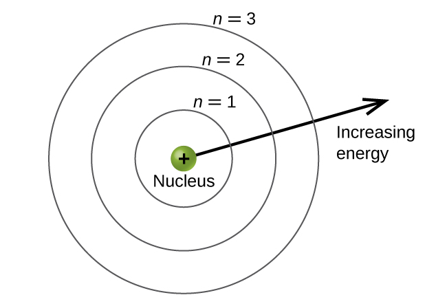
The principal energy levels are labeled with an n value, where n = 1, 2, 3, …. Generally speaking, the energy of an electron in an atom is greater for greater values of n and as the n value increases, so does the distance from the nucleus of the atom. This number, n, is referred to as the principal quantum number. The principal quantum number defines the location of the energy level and is essentially the same concept as the n in the Bohr atom description. Another name for the principal quantum number is the shell number. The spin quantum numbershells of an atom can be thought of concentric circles radiating out from the nucleus. The electrons that belong to a specific shell are most likely to be found within the corresponding circular area. The further we proceed from the nucleus, the higher the shell number, and so the higher the energy level (Figure 10.4a). The positively charged protons in the nucleus stabilize the electronic orbitals by electrostatic attraction between the positive charges of the protons and the negative charges of the electrons. So the further away the electron is from the nucleus, the greater the energy it has.
This quantum mechanical model for where electrons reside in an atom can be used to look at electronic transitions, the events when an electron moves from one energy level to another. As postulated by Bohr, if the transition is to a higher energy level, energy is absorbed, and the energy change has a positive value. To obtain the amount of energy necessary for the transition to a higher energy level, a photon of light is absorbed by the atom. A transition to a lower energy level involves a release of energy, and the discrete energy change is negative. This process is accompanied by emission of a photon by the atom. The following equation summarizes these relationships and is based on the hydrogen atom:
The values nf and ni are the final and initial energy states of the electron. To review calculations of such energy changes, see examples provided in Chapter 10.2 – The Bohr Atom .
The principal quantum number is one of three quantum numbers used to characterize an orbital. An atomic orbital, however, is distinct from Bohr’s orbit analogy where the electron was thought to move around the nucleus in circular, defined orbits. Instead, and atomic orbital is a general region in an atom within which an electron is most probable to reside or be found in a given instant. The quantum mechanical model specifies the probability of finding an electron in the three-dimensional space around the nucleus and is based on solutions of the Schrödinger equation. It does not provide the precise path taken by an electron. In addition, the principal quantum number defines the energy of an electron in a hydrogen or hydrogen-like atom or an ion (an atom or an ion with only one electron) and the general region in which discrete energy levels of electrons in a multi-electron atoms and ions are located.
Angular Momentum Quantum Number
Another quantum number is l, the angular momentum quantum number. It is an integer that defines the shape of the orbital, and takes on the values, l = 0, 1, 2, …, n – 1. This means that an orbital with n = 1 can have only one value of l, l = 0 (one orbital shape), whereas n = 2 permits l = 0 and l = 1 (two orbital shapes) and so on. The principal quantum number defines the general size and energy of the orbital. The l value specifies the shape of the orbital. Orbitals with the same value of l form a subshell. In addition, the greater the angular momentum quantum number, the greater is the angular momentum of an electron at this orbital.
Orbitals with l = 0 are called s orbitals (or the s subshells). The value l = 1 corresponds to the p orbitals. For a given n, p orbitals constitute a p subshell (e.g., 3p if n = 3). The orbitals with l = 2 are called the d orbitals, followed by the l = 3, called the f orbitals. There are higher values we will not consider, as introductory chemistry courses typically focus on s, p, d and sometimes f orbitals.
There are certain distances from the nucleus at which the probability density of finding an electron located at a particular orbital is zero. In other words, the value of the wave function ψ is zero at this distance for this orbital. Such a value of radius r is called a radial node, which is the spherical surface region where the probability of finding an electron is zero. The number of radial nodes in an orbital is n – l – 1.
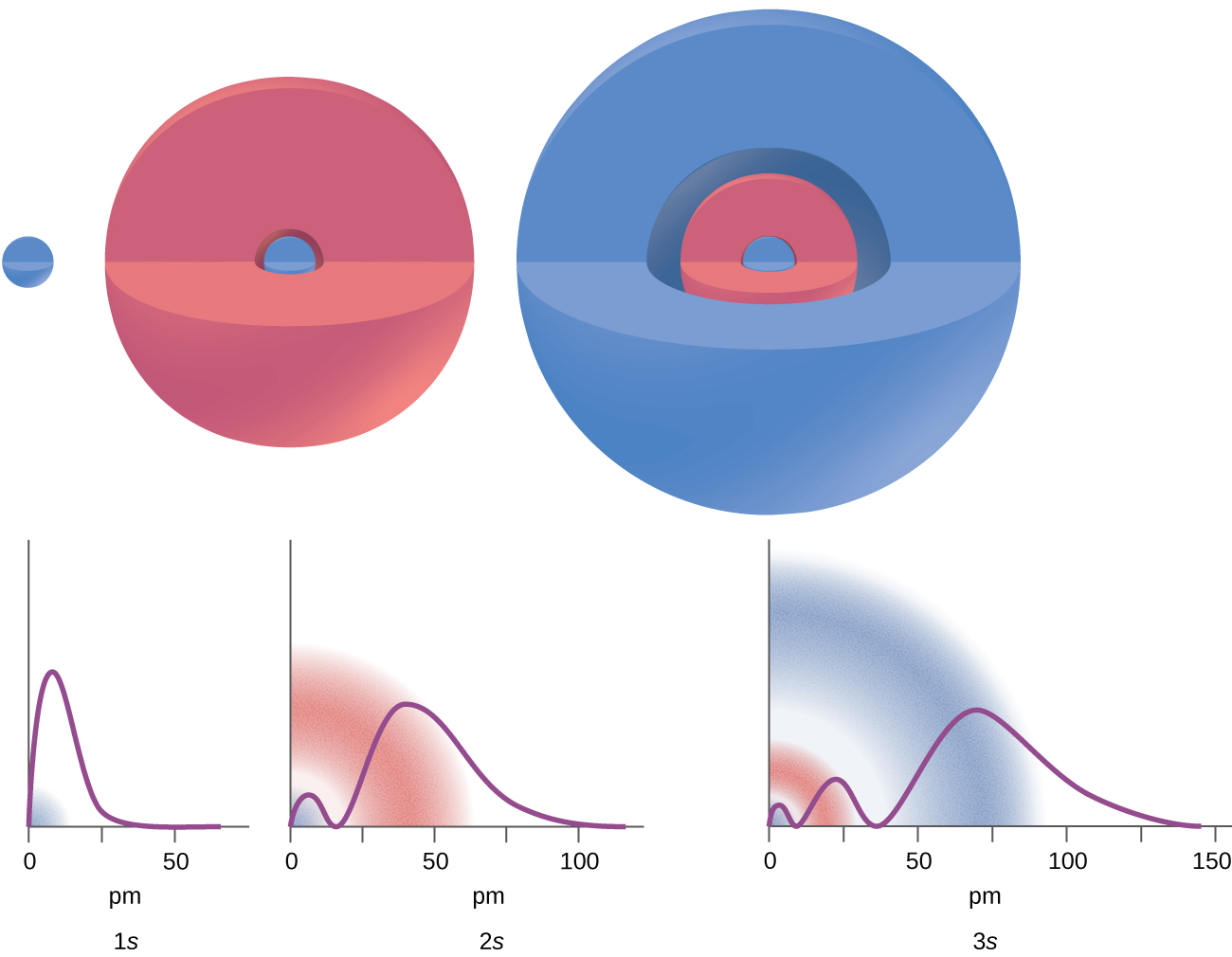
Consider the examples in Figure 10.4b. The orbitals depicted are of the s type (which were determined to be sphere shaped probability orbital shapes), thus l = 0 for all of them. It can be seen from the graphs of the probability densities that for 1s (n = 1) there are 1 – 0 – 1 = 0 places where the density is zero (nodes). For 2s (n = 2) there are 2 – 0 – 1 = 1 node, and for the 3s orbitals (n = 3) there are 3 – 0 – 1 = 2 nodes.
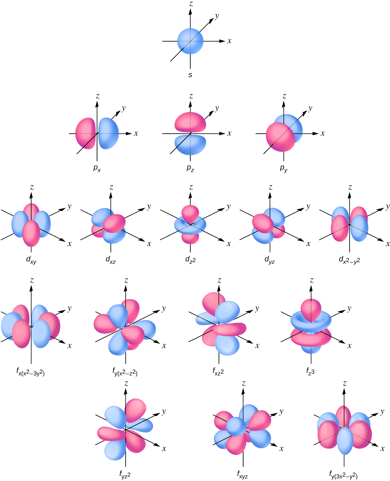
It was determined that the s subshell electron density distribution is spherical and the p subshell has a dumbbell shape. The d and f orbitals are more complex. These shapes represent the three-dimensional regions within which the electron is likely to be found (Figure 10.4c).
If an electron has an angular momentum (l ≠ 0), (as it will in p, d, f orbitals), then this vector can point in different directions. In addition, the z component of the angular momentum can have more than one value. This means that if a magnetic field is applied in the z direction, orbitals with different values of the z component of the angular momentum will have different energies resulting from interacting with the field. This provides the third quantum numbers, the magnetic quantum number, called ml,
Magnetic Quantum Number
The magnetic quantum number (ml) specifies the z component of the angular momentum for a particular orbital. For example, for an s orbital, l = 0, and the only value of ml is zero. For p orbitals, l = 1, and ml can be equal to –1, 0, or +1. Generally speaking, ml can be equal to –l, –(l – 1), …, –1, 0, +1, …, (l – 1), l. The total number of possible orbitals with the same value of l (a subshell) is 2l + 1. Thus, there is one s-orbital for ml = 0, there are three p-orbitals for ml = 1, five d-orbitals for ml = 2, seven f-orbitals for ml = 3, and so forth.
In summary, the principal quantum number defines the general value of the electronic energy, the angular momentum quantum number determines the shape of the orbital, and the magnetic quantum number specifies number of orientations of the orbital in space, as can be seen in Figure 10.4c.
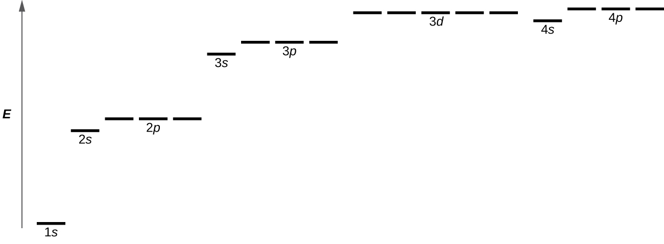
Figure 10.4d illustrates the energy levels for various orbitals. The number before the orbital name (such as 2s, 3p, and so forth) stands for the principal quantum number, n. The letter in the orbital name defines the subshell with a specific angular momentum quantum number l = 0 for s orbitals, 1 for p orbitals, 2 for d orbitals. Finally, there are more than one possible orbitals for l ≥ 1 (p, d, and f orbitals), each corresponding to a specific orientation, value of ml. Figure 10.4d illustrates the concept of degeneracy, electron orbitals having the same energy levels. In the case of a hydrogen atom or a one-electron ion (such as He+, Li2+, and so on), energies of all the orbitals with the same n are the same. In this case, the energy levels for the same principle quantum number, n, are called degenerate energy levels. However, in atoms with more than one electron, this degeneracy is eliminated by the electron–electron interactions, and orbitals that belong to different subshells in the same energy level have different energies, as shown on Figure 10.4d. For instance, an electron in the 2s orbital has lower energy than one in any of the three 2p orbitals. Orbitals of the same subshell (l value) are still degenerate and have the same energy (for example any of the three 2p subshells will have the same energy).
Spin Quantum Number
While the three quantum numbers discussed in the previous paragraphs work well for describing electron orbitals, some experiments showed that they were not sufficient to explain all observed results. It was demonstrated in the 1920s that when hydrogen-line spectra are examined at extremely high resolution, some lines are actually not single peaks but, rather, pairs of closely spaced lines. This is the so-called fine structure of the spectrum, and it implies that there are additional small differences in energies of electrons even when they are located in the same orbital. These observations led Samuel Goudsmit and George Uhlenbeck to propose that electrons have a fourth quantum number. They called this the spin quantum number, or ms.
The other three quantum numbers, n, l, and ml, are properties of specific atomic orbitals that also define in what part of the space an electron is most likely to be located. Orbitals are a result of solving the Schrödinger equation for electrons in atoms. The electron spin is a different kind of property. It is a completely quantum phenomenon with no analogues in the classical realm. In addition, it cannot be derived from solving the Schrödinger equation and is not related to the normal spatial coordinates (such as the Cartesian x, y, and z). Electron spin describes an intrinsic electron “rotation” or “spinning.” Each electron acts as a tiny magnet or a tiny rotating object with an angular momentum, even though this rotation cannot be observed in terms of the spatial coordinates.
The magnitude of the overall electron spin can only have one value, and an electron can only “spin” in one of two quantized states. One is termed the α state, with the z component of the spin being in the positive direction of the z axis. This corresponds to the spin quantum number [latex]m_s = \frac{1}{2}[/latex]. The other is called the β state, with the z component of the spin being negative and [latex]m_s = -\frac{1}{2}[/latex]. Any electron, regardless of the atomic orbital it is located in, can only have one of those two values of the spin quantum number. The energies of electrons having [latex]m_s = - \frac{1}{2}[/latex] and [latex]m_s = \frac{1}{2}[/latex] are different if an external magnetic field is applied.
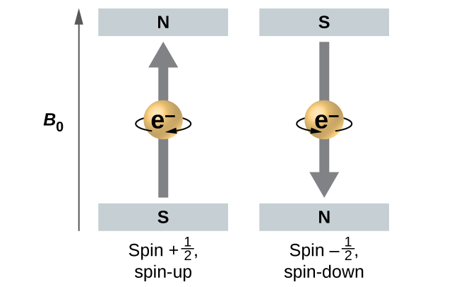
Figure 10.4e illustrates this phenomenon. An electron acts like a tiny magnet. Its moment is directed up (in the positive direction of the z axis) for the [latex]\frac{1}{2}[/latex] spin quantum number and down (in the negative z direction) for the spin quantum number of [latex]- \frac{1}{2}[/latex]. A magnet has a lower energy if its magnetic moment is aligned with the external magnetic field (the left electron on Figure 10.4e) and a higher energy for the magnetic moment being opposite to the applied field. This is why an electron with [latex]m_s = \frac{1}{2}[/latex] has a slightly lower energy in an external field in the positive z direction, and an electron with [latex]m_s = -\frac{1}{2}[/latex] has a slightly higher energy in the same field. This is true even for an electron occupying the same orbital in an atom. A spectral line corresponding to a transition for electrons from the same orbital but with different spin quantum numbers has two possible values of energy; thus, the line in the spectrum will show a fine structure splitting.
The Pauli Exclusion Principle
An electron in an atom is completely described by four quantum numbers: n, l, ml, and ms. The first three quantum numbers define the orbital and the fourth quantum number describes the intrinsic electron property called spin. An Austrian physicist Wolfgang Pauli formulated a general principle that gives the last piece of information that we need to understand the general behaviour of electrons in atoms. The Pauli exclusion principle can be formulated as follows: No two electrons in the same atom can have exactly the same set of all the four quantum numbers. What this means is that electrons can share the same orbital (the same set of the quantum numbers n, l, and ml), but only if their spin quantum numbers, ms, have different values. Since the spin quantum number can only have two values ([latex]\pm \frac{1}{2}[/latex]), no more than two electrons can occupy the same orbital (and if two electrons are located in the same orbital, they must have opposite spins). Therefore, any atomic orbital can be populated by only zero, one, or two electrons.
The properties and meaning of the quantum numbers of electrons in atoms are briefly summarized in Table 10.4a.
| Name | Symbol | Allowed values | Physical meaning |
|---|---|---|---|
| principal quantum number | n | 1, 2, 3, 4, …. | shell, the general region for the value of energy for an electron on the orbital; principal energy level |
| angular momentum or azimuthal quantum number | l | 0 ≤ l ≤ n – 1 | subshell, the shape of the orbital (s, p, d, f ….) |
| magnetic quantum number | ml | – l ≤ ml ≤ l | orientation of the orbital |
| spin quantum number | ms | [latex]\frac{1}{2}[/latex], [latex]- \frac{1}{2}[/latex] | direction of the intrinsic quantum “spinning” of the electron |
The quantum (wave) mechanical model of the atom was devised. Electrons occupy orbitals, which are probability fields or spaces around the nucleus of an atom where an electron is likely to be found. Important criteria was established in developing this modern atomic theory:
- Atoms have a series of energy levels called principal energy levels, which are designated by whole numbers (n = 1, 2, 3, ….).
- The energy of the level increases as the value of n increases.
- Each principal energy level contains one or more types of orbitals, called subshells.
- The number of subshells present in a given principal energy level equals n. For example: Principal energy level 4 (n = 4) has 4 subshells including s, p, d and f
- The n value is always used to label the orbitals of a given principal level and is followed by a letter that indicates the type (shape) of the orbital (For example: 1s, 2p, 3d ….).
- An orbital can be empty or it can contain one or two electrons, but never more than two. If two electrons occupy the same orbital, they must have opposite spins.
- The shape of an orbital does not indicate the specific details of electron movement (how it moves in a given orbital). It gives the probability distribution for where an electron is most likely to be found in that orbital.
- The total number of orbitals in a given shell (principal energy level) is 2n and the maximum number of electrons in each shell (principal energy level) is 2n2.
The properties of the principal energy levels (n = 1-4), subshells, and capacity of electrons in each subshell and energy level is summarized in Table 10.4b.
| Principal Energy Level (n) | Type of Subshell (l) | Number of Orbitals per Type of Subshell (ml) | Orbital Name | Maximum Number of Electrons in each Subshell | Maximum Number of Electrons in each Principal Energy Level (2n2) |
|---|---|---|---|---|---|
| 1 | s (0) | 1 (0) | 1s | 2 | 2 |
| 2 | s (0) | 1 (0) | 2s | 2 | |
| 2 | p (1) | 3 (-1, 0, +1) | 2p | 6 | 8 |
| 3 | s (0) | 1 (0) | 3s | 2 | |
| 3 | p (1) | 3 (-1, 0, +1) | 3p | 6 | |
| 3 | d (2) | 5 (-2, -1, 0, +1, +2) | 3d | 10 | 18 |
| 4 | s (0) | 1 (0) | 4s | 2 | |
| 4 | p (1) | 3 (-1, 0, +1) | 4p | 6 | |
| 4 | d (2) | 5 (-2, -1, 0, +1, +2) | 4d | 10 | |
| 4 | f (3) | 7 (-3, -2, -1, 0, +1, +2, +3) | 4f | 14 | 32 |
Source: “Table 10.4b” by Jackie MacDonald is licensed under CC BY-NC-SA 4.0.
For a video summary on quantum numbers and atomic orbitals as well as an introduction to electron orbital filling watch Quantum Numbers, Atomic Orbitals, and Electron Configurations (8min 41s)
Video Source: Professor Dave Explains (2015, August 31). Quantum numbers, atomic orbitals, and electron configurations [Video]. YouTube.
Example 10.4a
Working with Shells and Subshells
Indicate the number of subshells, the number of orbitals in each subshell, and the values of l and ml for the orbitals in the n = 4 shell of an atom. How many total orbitals are in principal energy level four (n = 4)
Solution
For n = 4, l can have values of 0, 1, 2, and 3. Thus, s, p, d, and f subshells are found in the n = 4 shell of an atom.
For l = 0 (the s subshell), ml can only be 0. Thus, there is only one 4s orbital.
For l = 1 (p-type orbitals), ml can have values of –1, 0, +1, so we find three 4p orbitals.
For l = 2 (d-type orbitals), ml can have values of –2, –1, 0, +1, +2, so we have five 4d orbitals.
When l = 3 (f-type orbitals), ml can have values of –3, –2, –1, 0, +1, +2, +3, and we can have seven 4f orbitals.
Thus, we find a total of (1+3+5+7) 16 orbitals in the n = 4 shell of an atom.
Exercise 10.4a
Working with Shells and Subshells
Identify the subshell in which electrons with the following quantum numbers are found: (a) n = 3, l = 1; (b) n = 4, l = 3; (c) n = 2, l = 0; (d) n = 5, l = 0; (e) n = 3, l = 2
Check Your Answer[1]
Example 10.4b
Maximum Number of Electrons – Electron Capacity
Calculate the maximum number of electrons that can occupy a shell with (a) n = 2, (b) n = 4, and (c) n as a variable. Note you are only looking at the orbitals with the specified n value, not those at lower energies.
Solution
(a) When n = 2, there are four orbitals (a single 2s orbital, and three orbitals labeled 2p). Since a maximum of two electrons can occupy the same orbital, these four orbitals can contain eight electrons. (4 orbitals x 2 electrons in each orbital = 8 electrons).
(b) When n = 4, there are four subshells of orbitals that we need to sum:
Again, each orbital holds two electrons, so 32 electrons can fit in this n = 4 shell (32 electrons can fit in the fourth energy level)
Alternatively, one could use the formula 2n2 = 2(4)2 = 2(16) = 32 electrons.
(c) The number of orbitals in any shell n will equal n2. There can be up to two electrons in each orbital, so the maximum number of electrons will be 2 × n2
Exercise 10.4b
Electron Capacity
Calculate the maximum number of electrons that can occupy a shell with
- n = 1
- n = 5
Check Your Answer[2]
Exercise 10.4c
Electron Capacity
If a shell contains a maximum of 32 electrons, what is the principal quantum number, n?
Check Your Answer[3]
Example 10.4c
Working with Quantum Numbers
Complete the following table for atomic orbitals using the following rules:
- The orbital designation is nl, where l = 0, 1, 2, 3, 4, … is mapped to the letter sequence s, p, d, f, g, …,
- The ml degeneracy is the number of orbitals within an l subshell, and so is 2l + 1 (there is one s orbital, three p orbitals, five d orbitals, seven f orbitals, and so forth).
- The number of radial nodes is equal to n – l – 1.
| Orbital | n | l | ml degeneracy | Radial nodes (no.) |
|---|---|---|---|---|
| 4f | [blank] | [blank] | [blank] | [blank] |
| [blank] | 4 | 1 | [blank] | [blank] |
| [blank] | 7 | [blank] | 7 | 3 |
| 5d | [blank] | [blank] | [blank] | [blank] |
Solution
| Orbital | n | l | ml degeneracy | Radial nodes (no.) |
|---|---|---|---|---|
| 4f | 4 | 3 | 7 | 0 |
| 4p | 4 | 1 | 3 | 2 |
| 7f | 7 | 3 | 7 | 3 |
| 5d | 5 | 2 | 5 | 2 |
Exercise 10.4d
How many orbitals have l = 2 and n = 3?
Check Your Answer[4]
Attribution & References
Except where otherwise noted, this page is adapted by Jackie MacDonald from:
- “6.3 Development of Quantum Theory” In Chemistry 2e (Open Stax) by Paul Flowers, Klaus Theopold, Richard Langley & William R. Robinson is licensed under CC BY 4.0. Access for free at Chemistry 2e (Open Stax) AND
- “3.3 Development of Quantum Theory” In General Chemistry 1 & 2 by Rice University, a derivative of Chemistry (Open Stax) by Paul Flowers, Klaus Theopold, Richard Langley & William R. Robinson and is licensed under CC BY 4.0. Access for free at Chemistry (OpenStax)
-
- n = 3 is the third energy level, l - 1 represents p orbital ANSWER is 3p;
- n = 4 is the fourth energy level, l - 3 represents f orbital ANSWER is 4f;
- n = 2 is the second energy level, l - 0 represents s orbital ANSWER is 2s;
- n = 5 is the fifth energy level, l - 0 represents s orbital ANSWER is 5s;
- n = 3 is the third energy level, l - 2 represents d orbital ANSWER is 3d
-
- 2n2 = 2(1)2 = 2 electrons fill the first principal energy level (shell, n = 1);
- 2n2 = 2(5)2 = 50 electrons fill the fifth principal energy level (shell, n = 5) ↵
- ANSWER n = 4 follow these steps to solve: 2n2 = 32 (divide each side by two) n2 = 16 (take the root of each side) n = 4; the fourth shell can has a capacity to fit 32 electrons ↵
- the five degenerate 3d orbitals ↵
the study of matter and its interactions with energy on the scale of atomic and subatomic particles. It includes the work of Schrodinger, Heisenberg and other scientists.
quantum number specifying the shell an electron occupies in an atom
quantum number distinguishing the different shapes of orbitals; it is also a measure of the orbital angular momentum
quantum number signifying the orientation of an atomic orbital around the nucleus; orbitals having different values of ml but the same subshell value of l have the same energy (are degenerate), but this degeneracy can be removed by application of an external magnetic field
number specifying the electron spin direction, either +1/2 or -1/2
set of orbitals with the same principal quantum number, n
mathematical function that describes the behavior of an electron in an atom (also called the wavefunction), it can be used to find the probability of locating an electron in a specific region around the nucleus, as well as other dynamical variables
set of orbitals in an atom with the same values of n and l
spherical region of space with high electron density, describes orbitals with l = 0. An electron in this orbital is called an s electron
written as: p orbitals
dumbbell-shaped region of space with high electron density, describes orbitals with l = 1. An electron in this orbital is called a p electron
written as: d orbitals
region of space with high electron density that is either four lobed or contains a dumbbell and torus shape; describes orbitals with l = 2. An electron in this orbital is called a d electron
electron orbitals having the same energy levels
specifies that no two electrons in an atom can have the same value for all four quantum numbers
