8.4 – Quantum Mechanics

Shortly after de Broglie published his ideas that the electron in a hydrogen atom could be better thought of as being a circular standing wave instead of a particle moving in quantized circular orbits, as Bohr had argued, Erwin Schrödinger extended de Broglie’s work by incorporating the de Broglie relation into a wave equation, deriving what is today known as the Schrödinger equation. When Schrödinger applied his equation to hydrogen-like atoms, he was able to reproduce Bohr’s expression for the energy and, thus, the Rydberg formula governing hydrogen spectra, and he did so without having to invoke Bohr’s assumptions of stationary states and quantized orbits, angular momenta, and energies; quantization in Schrödinger’s theory was a natural consequence of the underlying mathematics of the wave equation. Like de Broglie, Schrödinger initially viewed the electron in hydrogen as being a physical wave instead of a particle, but where de Broglie thought of the electron in terms of circular stationary waves, Schrödinger properly thought in terms of three-dimensional stationary waves, or wavefunctions, represented by the Greek letter psi, ѱ. A few years later, Max Born proposed an interpretation of the wavefunction ѱ that is still accepted today: Electrons are still particles, and so the waves represented by ѱ are not physical waves but, instead, are complex probability amplitudes. The square of the magnitude of a wavefunction ∣ѱ∣² describes the probability of the quantum particle being present near a certain location in space. This means that wavefunctions can be used to determine the distribution of the electron’s density with respect to the nucleus in an atom. In the most general form, the Schrödinger equation can be written as:

Ĥѱ＝Eѱ

Equation 8.4.1 Schrödinger Equation

Schrödinger’s work, as well as that of Heisenberg and many other scientists following in their footsteps, is generally referred to as quantum mechanics.

You may also have heard of Schrödinger because of his famous thought experiment. This story explains the concepts of superposition and entanglement as related to a cat in a box with poison.

Understanding Quantum Theory of Electrons in Atoms

The goal of this section is to understand the electron orbitals (location of electrons in atoms), their different energies, and other properties. The use of quantum theory provides the best understanding of these topics. This knowledge is a precursor to chemical bonding.

As was described previously, electrons in atoms can exist only on discrete energy levels but not between them. It is said that the energy of an electron in an atom is quantized, that is, it can be equal only to certain specific values and can jump from one energy level to another but not transition smoothly or stay between these levels.

The energy levels are labeled with an n value, where n = 1, 2, 3, …. Generally speaking, the energy of an electron in an atom is greater for greater values of n. This number, n, is referred to as the principal quantum number. The principal quantum number defines the location of the energy level. It is essentially the same concept as the n in the Bohr atom description. Another name for the principal quantum number is the shell number. The shells of an atom can be thought of concentric spheres radiating out from the nucleus. The electrons that belong to a specific shell are most likely to be found within the corresponding circular area. The further we proceed from the nucleus, the higher the shell number, and so the higher the energy level (Figure 8.4.1.). The positively charged protons in the nucleus stabilize the electronic orbitals by electrostatic attraction between the positive charges of the protons and the negative charges of the electrons. So the further away the electron is from the nucleus, the greater the energy it has.

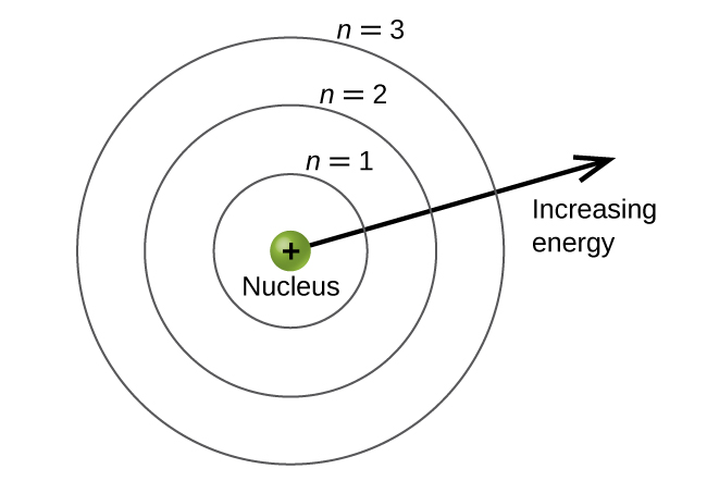
Figure 8.4.1. Different shells are numbered by principal quantum numbers.

This quantum mechanical model for where electrons reside in an atom can be used to look at electronic transitions, the events when an electron moves from one energy level to another. If the transition is to a higher energy level, energy is absorbed, and the energy change has a positive value. To obtain the amount of energy necessary for the transition to a higher energy level, a photon is absorbed by the atom. A transition to a lower energy level involves a release of energy, and the energy change is negative. This process is accompanied by emission of a photon by the atom. The following equation summarizes these relationships and is based on the hydrogen atom:

ΔE = E_final – E_initial

= -2.18 × 10^-18 ((1 / n_f²) – (1 / n₁²)) J

The values n_f and n_i are the final and initial energy states of the electron. The example calculating the energy and wavelength of electron transitions in a one–electron (Bohr) system in topic 8.2 of the chapter demonstrates calculations of such energy changes.

The principal quantum number is one of three quantum numbers used to characterize an orbital. An atomic orbital, which is distinct from an orbit, is a general region in an atom within which an electron is most probable to reside. The quantum mechanical model specifies the probability of finding an electron in the three-dimensional space around the nucleus and is based on solutions of the Schrödinger equation. In addition, the principal quantum number defines the energy of an electron in a hydrogen or hydrogen-like atom or an ion (an atom or an ion with only one electron) and the general region in which discrete energy levels of electrons in a multi-electron atoms and ions are located.

Another quantum number is ℓ (lowercase letter L), the angular momentum quantum number. It is an integer that defines the shape of the orbital, and takes on the values, l = 0, 1, 2, …, n – 1. This means that an orbital with n = 1 can have only one value of l, l = 0, whereas n = 2 permits l = 0 and l = 1, and so on. The principal quantum number defines the general size and energy of the orbital. The l value specifies the shape of the orbital. Orbitals with the same value of l form a subshell. In addition, the greater the angular momentum quantum number, the greater is the angular momentum of an electron at this orbital.

Orbitals with l = 0 are called s orbitals (or the s subshells). The value l = 1 corresponds to the p orbitals. For a given n, p orbitals constitute a p subshell (e.g., 3p if n = 3). The orbitals with l = 2 are called the d orbitals, followed by the f-, g-, and h-orbitals for l = 3, 4, 5, and there are higher values we will not consider.

There are certain distances from the nucleus at which the probability density of finding an electron located at a particular orbital is zero. In other words, the value of the wavefunction ψ is zero at this distance for this orbital. Such a value of radius r is called a radial node. The number of radial nodes in an orbital is n – l – 1.

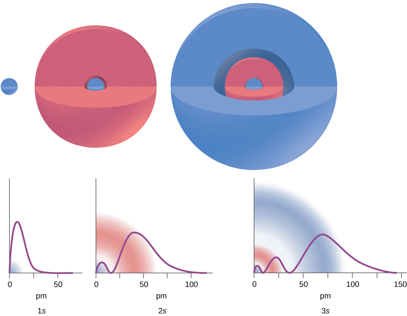
Figure 8.4.2. The graphs show the probability (y axis) of finding an electron for the 1s, 2s, 3s orbitals as a function of distance from the nucleus.

Consider the examples in Figure 8.4.2. The orbitals depicted are of the s type, thus l = 0 for all of them. It can be seen from the graphs of the probability densities that there are 1 – 0 – 1 = 0 places where the density is zero (nodes) for 1s (n = 1), 2 – 0 – 1 = 1 node for 2s, and 3 – 0 – 1 = 2 nodes for the 3s orbitals.

The s subshell electron density distribution is spherical and the p subshell has a dumbbell shape. The d and f orbitals are more complex. These shapes represent the three-dimensional regions within which the electron is likely to be found.

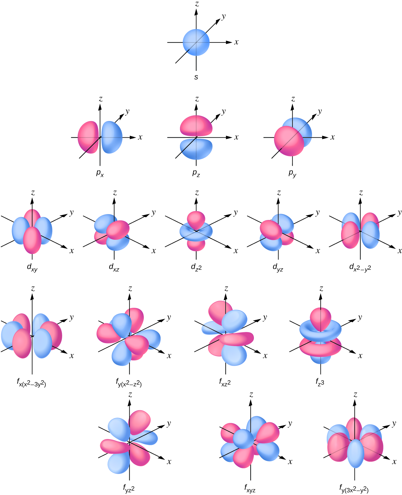
Figure 8.4.3. Shapes of s, p, d, and f orbitals.

If an electron has an angular momentum (l ≠ 0), then this vector can point in different directions. In addition, the z component of the angular momentum can have more than one value. This means that if a magnetic field is applied in the z direction, orbitals with different values of the z component of the angular momentum will have different energies resulting from interacting with the field. The magnetic quantum number, called m_ℓ, specifies the z component of the angular momentum for a particular orbital. For example, for an s orbital, l = 0, and the only value of m_l is zero. For p orbitals, l = 1, and m_l can be equal to –1, 0, or +1. Generally speaking, m_l can be equal to –l, –(l – 1), …, –1, 0, +1, …, (l – 1), l. The total number of possible orbitals with the same value of l (a subshell) is 2l + 1. Thus, there is one s-orbital for l = 0, there are three p-orbitals for l = 1, five d-orbitals for l = 2, seven f-orbitals for l = 3, and so forth. The principal quantum number defines the general value of the electronic energy. The angular momentum quantum number determines the shape of the orbital. And the magnetic quantum number specifies orientation of the orbital in space, as can be seen in Figure 8.4.3.

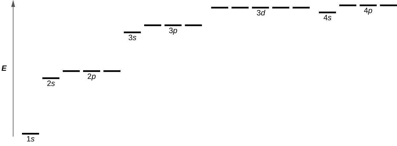
Figure 8.4.4. The chart shows the energies of electron orbitals in a multi-electron atom.

Figure 8.4.4. illustrates the energy levels for various orbitals. The number before the orbital name (such as 2s, 3p, and so forth) stands for the principal quantum number, n. The letter in the orbital name defines the subshell with a specific angular momentum quantum number l = 0 for s orbitals, 1 for p orbitals, 2 for d orbitals. Finally, there are more than one possible orbitals for l ≥ 1, each corresponding to a specific value of m_l. In the case of a hydrogen atom or a one-electron ion (such as He⁺, Li²⁺, and so on), energies of all the orbitals with the same n are the same. This is called a degeneracy, and the energy levels for the same principal quantum number, n, are called degenerate orbitals. However, in atoms with more than one electron, this degeneracy is eliminated by the electron–electron interactions, and orbitals that belong to different subshells have different energies, as shown on Figure 8.4.4. Orbitals within the same subshell (for example ns, np, nd, nf, such as 2p, 3s) are still degenerate and have the same energy.

While the three quantum numbers discussed in the previous paragraphs work well for describing electron orbitals, some experiments showed that they were not sufficient to explain all observed results. It was demonstrated in the 1920s that when hydrogen-line spectra are examined at extremely high resolution, some lines are actually not single peaks but, rather, pairs of closely spaced lines. This is the so-called fine structure of the spectrum, and it implies that there are additional small differences in energies of electrons even when they are located in the same orbital. These observations led Samuel Goudsmit and George Uhlenbeck to propose that electrons have a fourth quantum number. They called this the spin quantum number, or m_s.

The other three quantum numbers, n, l, and m_l, are properties of specific atomic orbitals that also define in what part of the space an electron is most likely to be located. Orbitals are a result of solving the Schrödinger equation for electrons in atoms. The electron spin is a different kind of property. It is a completely different quantum phenomenon with no analogues in the classical realm. In addition, it cannot be derived from solving the Schrödinger equation and is not related to the normal spatial coordinates (such as the Cartesian x, y, and z). Electron spin describes an intrinsic electron “rotation” or “spinning.” Each electron acts as a tiny magnet or a tiny rotating object with an angular momentum, or as a loop with an electric current, even though this rotation or current cannot be observed in terms of spatial coordinates.

The magnitude of the overall electron spin can only have one value, and an electron can only “spin” in one of two quantized states. Think of a planet for example, regardless of the position of direction of the planetary axis, it can only rotate in two directions: “clockwise” or “counterclockwise”. One of the two quantized states is termed the α state, with the z component of the spin being in the positive direction of the z axis. This corresponds to the spin quantum number m_s​ = 12. The other is called the β state, with the z component of the spin being negative and m_s ​= -12. Any electron, regardless of the atomic orbital it is located in, can only have one of those two values of the spin quantum number. The energies of electrons having m_s​ = -12 and m_s = 12 are different if an external magnetic field is applied.

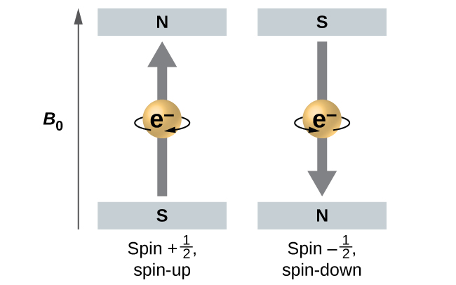
Figure 8.4.5. Electrons with spin values ±12 in an external magnetic field.

Figure 8.4.5. illustrates this phenomenon. An electron acts like a tiny magnet. Its moment is directed up (in the positive direction of the z axis) for the 12 spin quantum number and down (in the negative z direction) for the spin quantum number of -12 (Note: the up and down directions are completely arbitrary, and are results of unanimous agreement to denote them as such). A magnet has a lower energy if its magnetic moment is aligned with the external magnetic field (the left electron on Figure 8.4.5.) and a higher energy for the magnetic moment being opposite to the applied field. This is why an electron with m_s = 12 has a slightly lower energy in an external field in the positive z direction, and an electron with m_s = -12 has a slightly higher energy in the same field. This is true even for an electron occupying the same orbital in an atom. A spectral line corresponding to a transition for electrons from the same orbital but with different spin quantum numbers has two possible values of energy; thus, the line in the spectrum will show a fine structure splitting.

★ Questions

1. How are the Bohr model and the quantum mechanical model of the hydrogen atom similar? How are they different?

2. What are the allowed values for each of the four quantum numbers: n, l, m_l, and ms?

3. Describe the properties of an electron associated with each of the following four quantum numbers: n, l, m_l, and ms.

4. Answer the following questions:

a) Without using quantum numbers, describe the differences between the shells, subshells, and orbitals of an atom.

b) How do the quantum numbers of the shells, subshells, and orbitals of an atom differ?

5. Identify the subshell in which electrons with the following quantum numbers are found:

a) n = 2, l = 1

b) n = 4, l = 2

c) n = 6, l = 0

6. Which of the subshells described in the previous question contain degenerate orbitals? How many degenerate orbitals are in each?

7. Identify the subshell in which electrons with the following quantum numbers are found:

a) n = 3, l = 2

b) n = 1, l = 0

c) n = 4, l = 3

8. Which of the subshells described in the previous question contain degenerate orbitals? How many degenerate orbitals are in each?

Answers

1. Both models have a central positively charged nucleus with electrons moving about the nucleus in accordance with the Coulomb electrostatic potential. The Bohr model assumes that the electrons move in circular orbits that have quantized energies, angular momentum, and radii that are specified by a single quantum number, n = 1, 2, 3, …, but this quantization is an ad hoc assumption made by Bohr to incorporate quantization into an essentially classical mechanics description of the atom. Bohr also assumed that electrons orbiting the nucleus normally do not emit or absorb electromagnetic radiation, but do so when the electron switches to a different orbit. In the quantum mechanical model, the electrons do not move in precise orbits (such orbits violate the Heisenberg uncertainty principle) and, instead, a probabilistic interpretation of the electron’s position at any given instant is used, with a mathematical function ψ called a wavefunction that can be used to determine the electron’s spatial probability distribution. These wavefunctions, or orbitals, are three-dimensional stationary waves that can be specified by three quantum numbers that arise naturally from their underlying mathematics (no ad hoc assumptions required): the principal quantum number, n (the same one used by Bohr), which specifies shells such that orbitals having the same n all have the same energy and approximately the same spatial extent; the angular momentum quantum number l, which is a measure of the orbital’s angular momentum and corresponds to the orbitals’ general shapes, as well as specifying subshells such that orbitals having the same l (and n) all have the same energy; and the orientation quantum number m, which is a measure of the z component of the angular momentum and corresponds to the orientations of the orbitals. The Bohr model gives the same expression for the energy as the quantum mechanical expression and, hence, both properly account for hydrogen’s discrete spectrum (an example of getting the right answers for the wrong reasons, something that many chemistry students can sympathize with), but gives the wrong expression for the angular momentum (Bohr orbits necessarily all have non-zero angular momentum, but some quantum orbitals [s orbitals] can have zero angular momentum).

2. n = 1,2,3,4…

l = 0 to (n-1)

m_l = -1 to +1

ms = -½ to +½

3. n determines the general range for the value of energy and the probable distances that the electron can be from the nucleus. l determines the shape of the orbital. m_l determines the orientation of the orbitals of the same l value with respect to one another. ms determines the spin of an electron.

4.

(a)

shell: set of orbitals in the same energy level

subshell: set of orbitals in the same energy level and same shape (s, p, d, or f)

orbital: can hold up to 2 electrons

(b)

shell: set of orbitals in the same energy level

subshell: set of orbitals in the same energy level and same shape (s, p, d, or f)

orbital: can hold up to 2 electrons

5. (a) 2p; (b) 4d; (c) 6s

6. (a) 3 orbitals; (b) 5 orbitals; (c) 1 orbital

7. (a) 3d; (b) 1s; (c) 4f

8. (a) 5 orbitals ;(b) 1 orbital ;(c) 7 orbitals