8.3 – Wave-Particle Duality of Matter & Energy
Einstein initially assumed that photons had zero mass, which made them a peculiar sort of particle indeed. In 1905, however, he published his special theory of relativity, which related energy and mass according to the following equation:
Equation 8.3.1 Energy Mass Relation
According to this theory, a photon of wavelength λ and frequency ν has a nonzero mass, which is given as follows:
Equation 8.3.2 Energy Mass Relation of Photon
That is, light, which had always been regarded as a wave, also has properties typical of particles, a condition known as wave–particle duality (a principle that matter and energy have properties typical of both waves and particles). Depending on conditions, light could be viewed as either a wave or a particle.
One of the first people to pay attention to the special behavior of the microscopic world was Louis de Broglie. He asked the question: If electromagnetic radiation can have particle-like character, can electrons and other submicroscopic particles exhibit wavelike character? In his 1925 doctoral dissertation, de Broglie extended the wave–particle duality of light that Einstein used to resolve the photoelectric-effect paradox to material particles. He predicted that a particle with mass m and velocity v (that is, with linear momentum p) should also exhibit the behavior of a wave with a wavelength value λ, given by this expression in which h is the familiar Planck’s constant:
λ = hmv = hp
Equation 8.3.3 Wavelength Momentum Equation
This is called the de Broglie wavelength. Unlike the other values of λ discussed in this chapter, the de Broglie wavelength is a characteristic of particles and other bodies, not electromagnetic radiation (note that this equation involves velocity [v, m/s], not frequency [ν, Hz]. Although these two symbols appear nearly identical, they mean very different things). Where Bohr had postulated the electron as being a particle orbiting the nucleus in quantized orbits, de Broglie argued that Bohr’s assumption of quantization can be explained if the electron is considered not as a particle, but rather as a circular standing wave such that only an integer number of wavelengths could fit exactly within the orbit (Figure 8.3.1.).
2πr = nλ, n = 1, 2, 3, …
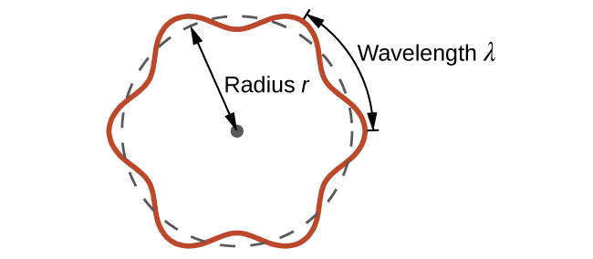
Figure 8.3.1. If an electron is viewed as a wave circling around the nucleus, an integer number of wavelengths must fit into the orbit for this standing wave behavior to be possible.
For a circular orbit of radius r, the circumference is 2πr, and so de Broglie’s condition is:
Since the de Broglie expression relates the wavelength to the momentum and, hence, velocity, this implies:
This expression can be rearranged to give Bohr’s formula for the quantization of the angular momentum:
Equation 8.3.4 Quantization of the Angular Momentum
Classical angular momentum L for a circular motion is equal to the product of the radius of the circle and the momentum of the moving particle p.
L = rp = rmv (for a circular motion)
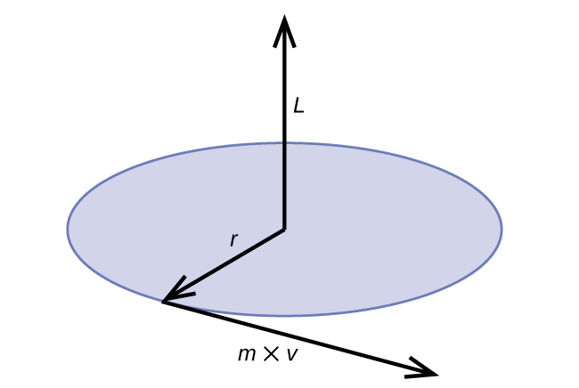
Figure 8.3.2. The diagram shows angular momentum for a circular motion.
Shortly after de Broglie proposed the wave nature of matter, two scientists at Bell Laboratories, C. J. Davisson and L. H. Germer, demonstrated experimentally that electrons can exhibit wavelike behavior by showing an interference pattern for electrons travelling through a regular atomic pattern in a crystal. The regularly spaced atomic layers served as slits, as used in other interference experiments. Since the spacing between the layers serving as slits needs to be similar in size to the wavelength of the tested wave for an interference pattern to form, Davisson and Germer used a crystalline nickel target for their “slits,” since the spacing of the atoms within the lattice was approximately the same as the de Broglie wavelengths of the electrons that they used. Figure 8.3.3. shows an interference pattern. It is strikingly similar to the interference patterns for light shown in the example determining the frequency and wavelength of radiation in topic 8.1. The wave–particle duality of matter can be seen in Figure 8.3.3. by observing what happens if electron collisions are recorded over a long period of time. Initially, when only a few electrons have been recorded, they show clear particle-like behavior, having arrived in small localized packets that appear to be random. As more and more electrons arrived and were recorded, a clear interference pattern that is the hallmark of wavelike behavior emerged. Thus, it appears that while electrons are small localized particles, their motion does not follow the equations of motion implied by classical mechanics, but instead it is governed by some type of a wave equation that governs a probability distribution even for a single electron’s motion. Thus the wave–particle duality first observed with photons is actually a fundamental behavior intrinsic to all quantum particles.
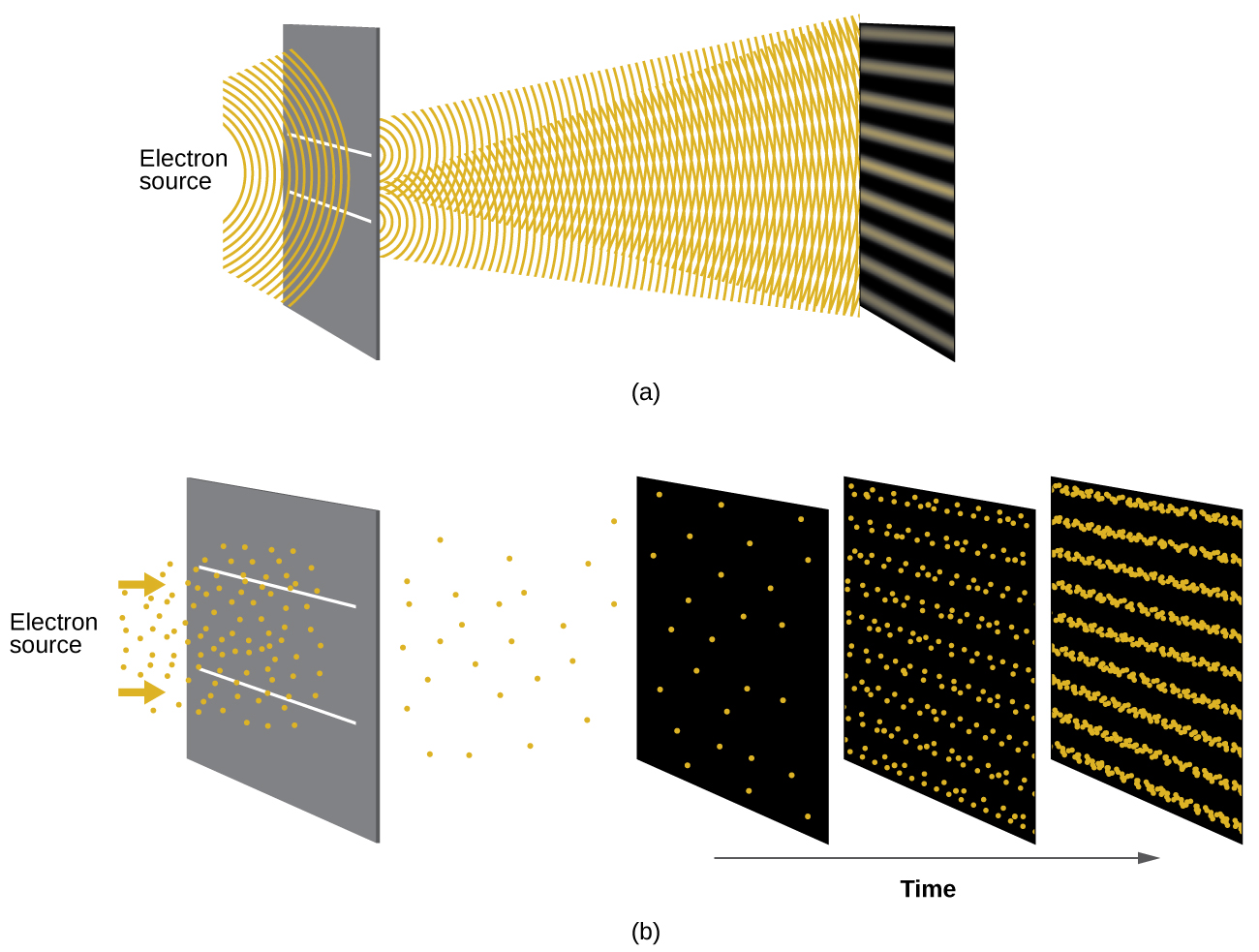
Figure 8.3.3. (a) The interference pattern for electrons passing through very closely spaced slits demonstrates that quantum particles such as electrons can exhibit wavelike behavior. (b) The experimental results illustrated here demonstrate the wave–particle duality in electrons. The electrons pass through very closely spaced slits, forming an interference pattern, with increasing numbers of electrons being recorded from the left image to the right. With only a few electrons recorded, it is clear that the electrons arrive as individual localized “particles,” but in a seemingly random pattern. As more electrons arrive, a wavelike interference pattern begins to emerge. Note that the probability of the final electron location is still governed by the wave-type distribution, even for a single electron, but it can be observed more easily if many electron collisions have been recorded.
View the Dr. Quantum – Double Slit Experiment cartoon for an easy-to-understand description of wave–particle duality and the associated experiments.
Example 8.3.1 – Calculating the Wavelength of a Particle
If an electron travels at a velocity of 1.000 × 10⁷ m s–1 and has a mass of 9.109 × 10⁻²⁸ g, what is its wavelength?
Solution
We can use de Broglie’s equation to solve this problem, but we first must do a unit conversion of Planck’s constant. You learned earlier that 1 J = 1 kg m2/s2. Thus, we can write h = 6.626 × 10⁻³⁴ J s as 6.626 × 10⁻³⁴ kg m2/s.
λ = hmv
= 6.626 × 10⁻³⁴ kgm2/s (9.109×10⁻³¹ kg)(1.000 × 10⁷ m/s)
=7.274 × 10⁻¹¹m
This is a small value, but it is significantly larger than the size of an electron in the classical (particle) view. This size is the same order of magnitude as the size of an atom. This means that electron wavelike behavior is going to be noticeable in an atom.
Check Your Learning 8.3.1 – Calculating the Wavelength of a Particle
Calculate the wavelength of a softball with a mass of 100 g traveling at a velocity of 35 m s–1, assuming that it can be modeled as a single particle.
Answer
1.9 × 10⁻³⁴ m. We never think of a thrown softball having a wavelength, since this wavelength is so small it is impossible for our senses or any known instrument to detect (strictly speaking, the wavelength of a real baseball would correspond to the wavelengths of its constituent atoms and molecules, which, while much larger than this value, would still be microscopically tiny). The de Broglie wavelength is only appreciable for matter that has a very small mass and/or a very high velocity.
Werner Heisenberg considered the limits of how accurately we can measure properties of an electron or other microscopic particles. He determined that there is a fundamental limit to how accurately one can measure both a particle’s position and its momentum simultaneously. The more accurately we measure the momentum of a particle, the less accurately we can determine its position at that time, and vice versa. This is summed up in what we now call the Heisenberg uncertainty principle: It is fundamentally impossible to determine simultaneously and exactly both the momentum and the position of a particle. For a particle of mass m moving with velocity vx in the x direction (or equivalently with momentum px), the product of the uncertainty in the position, Δx, and the uncertainty in the momentum, Δpx , must be greater than or equal to ℏ / 2 (recall that ℏ = h / (2π), the value of Planck’s constant divided by 2π).
Δx × Δpx = (Δx)(mΔv) ≥ ♄ / 2
Equation 8.3.5 Heisenberg Uncertainty Principle
This equation allows us to calculate the limit to how precisely we can know both the simultaneous position of an object and its momentum. For example, if we improve our measurement of an electron’s position so that the uncertainty in the position (Δx) has a value of, say, 1 pm (10–12 m, about 1% of the diameter of a hydrogen atom), then our determination of its momentum must have an uncertainty with a value of at least
Δp = mΔv = h(2Δx) = (1.055 × 10⁻³⁴ kgm2 / s)(2 × 1 × 10-12 m) = 5 × 10-23 kgm / s
The value of ħ is not large, so the uncertainty in the position or momentum of a macroscopic object like a baseball is too insignificant to observe. However, the mass of a microscopic object such as an electron is small enough that the uncertainty can be large and significant.
It should be noted that Heisenberg’s uncertainty principle is not just limited to uncertainties in position and momentum, but it also links other dynamical variables. For example, when an atom absorbs a photon and makes a transition from one energy state to another, the uncertainty in the energy and the uncertainty in the time required for the transition are similarly related, as ΔE Δt ≥ ℏ / 2. As will be discussed later, even the vector components of angular momentum cannot all be specified exactly simultaneously.
Heisenberg’s principle imposes ultimate limits on what is knowable in science. The uncertainty principle can be shown to be a consequence of wave–particle duality, which lies at the heart of what distinguishes modern quantum theory from classical mechanics. Recall that the equations of motion obtained from classical mechanics are trajectories where, at any given instant in time, both the position and the momentum of a particle can be determined exactly. Heisenberg’s uncertainty principle implies that such a view is untenable in the microscopic domain and that there are fundamental limitations governing the motion of quantum particles. This does not mean that microscopic particles do not move in trajectories, it is just that measurements of trajectories are limited in their precision. In the realm of quantum mechanics, measurements introduce changes into the system that is being observed.
Read this article that describes a recent macroscopic demonstration of the uncertainty principle applied to microscopic objects.
★ Questions
1. Calculate the wavelength of a baseball, which has a mass of 149 g and a speed of 100 mi/h.
2. Calculate the wavelength of a neutron that is moving at 3.00 × 10³ m/s (in Å or pm).
3. Calculate the wavelength (in meters) associated with a 42 g baseball with speed of 80 m/s.
4. Calculate the de Broglie wavelengths of the following:
a) An 8g bullet with velocity 340ms-1.
b) A 10-5g particle with velocity 10-5ms-1.
c) A 10-8g particle with velocity 10-8ms-1.
d) An electron moving with velocity 4.8 x 10⁶ ms-1.
Answers
1. 9.95 x 10⁻³⁵
2. 1.32 Å, or 132 pm
3. 1.97 x 10⁻³⁴ m
4. (a) 2.44 x 10⁻³³ (b) 6.626 x 10⁻²¹ (c) 6.626 x 10⁻¹⁵ (d) 1.52 x 10⁻¹⁰
Rule stating that it is impossible to exactly determine both certain conjugate dynamical properties such as the momentum and the position of a particle at the same time. The uncertainty principle is a consequence of quantum particles exhibiting wave–particle duality
