Solutions: Case Study – Automation in Fast Food
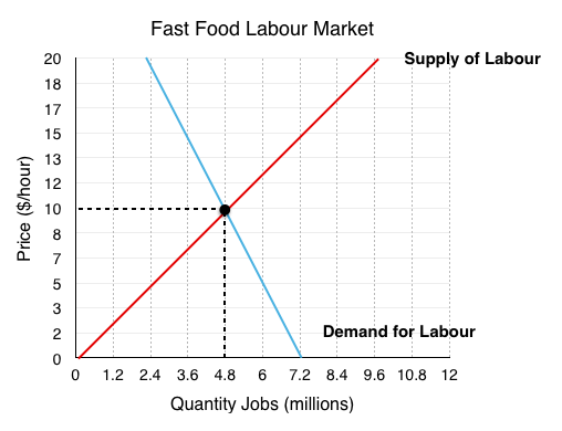
1. A supply and demand curve for the fast food labour market is presented below, label the equilibrium price and quantity.
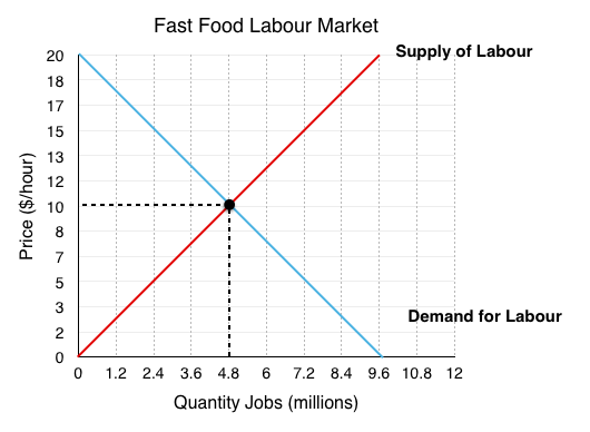
Since Firms demand the labour, they represent the demand side of the market.
Since Job Searchers supply the labour, they represent the supply side of the market.
The equilibrium occurs at the intersection of supply and demand, in this case @ EP = $10/hr, EQ = 4.8 million workers employed.
2. What is consumer and producer surplus? Market surplus?
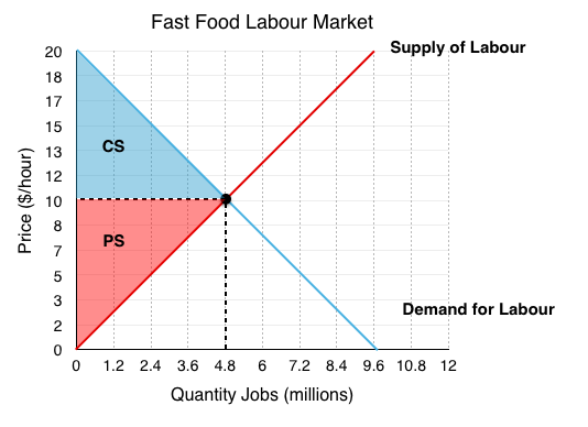
Consumer Surplus
It is important to understand that firms are the consumers in this situation since they demand and ‘consume’ labour. Recall consumer surplus is the difference between willingness to pay and the wage they pay paid. This is equal to the area labelled CS represented by the blue triangle in the figure above.
[latex]\frac{\left(20-10\right)\times \left(4.8\right)}{2}[/latex] = $24 million
Producer Surplus
In this contexts the producers are the job searchers/workers since they ‘produce’ labour for the firms to buy. Producer surplus is the difference between the marginal cost of labour (commuting, opportunity cost, etc) and the wage.
[latex]\frac{\left(10-0\right)\times \left(4.8\right)}{2}[/latex] = $24 million
Market Surplus
Market surplus is just consumer surplus + producer surplus.
$24 million + $24 million = $48 million
3. Assume the government passes policy introducing a $15 minimum wage. Label the new quantity demanded, and quantity supplied. Is there a shortage or a surplus of labour?
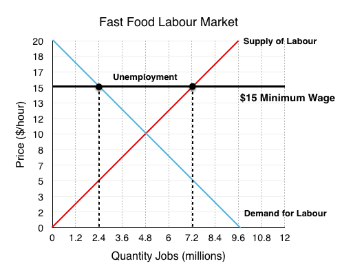
A minimum wage is the same as a price floor, a government policy that restricts price from falling below the mandated level. In this case price is wage. At a wage of $15/hour quantity of labour demanded = 2.4 million, whereas quantity of labour supplied = 7.2 million. The resulting unemployment represents a surplus of workers in the market.
4. What are the two effects of the minimum wage on workers? What is the net change in surplus?
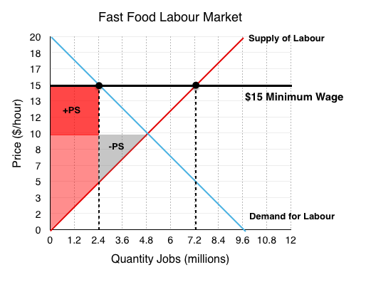
When you have a price change from equilibrium two things happen – a transfer and a deadweight loss. In this example the two mean very different things for consumers.
The transfer
There are clear benefits for the minimum wage if you keep your job. For the 2.4 million workers in this situation who go from receiving a wage of $10/hour to $15/hour, their surplus increases. This increase is represented by the highlighted red region labelled +PS.
($15-$10)*(2.4) = +$12 million
The deadweight loss
The workers who lose their jobs from the policy are less happy. In this case 2.4 million workers are now unable to find work. Note that these are the workers who faced the highest marginal cost of labour, the decrease in surplus is represented by the grey region labelled -PS.
[latex]\frac{\left(10-5\right)\times \left(2.4\right)}{2}[/latex] = -$6 million.
The net change in surplus for workers is +$6 million ($12 million – $6 million)
5. What is the deadweight loss from this policy?
Even though workers gain from the policy, we cannot forget about the firms!
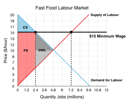
Although the breakdown of the firms is not represented, we know that the ‘transfer’ from question 4 was coming out of the pockets of firms. For deadweight loss, this is irrelevant since is is just a redistribution of surplus.
What we are interested in are the firms who are no longer employing workers, going out of business because workers are too expensive. This is represented by the darker of the two grey regions.
[latex]\frac{\left(15-10\right)\times \left(2.4\right)}{2}[/latex] = $6 million
Adding the two DWL areas together, we find the minimum wage resulted in inefficiencies of $12 million ($6 million + $6 million)
6. A new supply and demand curve for the fast food labour market is presented below with a more inelastic supply curve, label the new equilibrium price and quantity.
The new equilibrium occurs where the supply curve intersects the new demand curve, in this case @ EP = $10/hr, EQ = 2.4 million workers employed.
Note that the equilibrium is the same, but the slope has changed, meaning the demand curve crosses through different points at every other quantity.
7. Assume the government again passes policy introducing a $15 minimum wage. Label the new quantity demanded, quantity supplied. Is there a shortage or a surplus of labour? By how much?
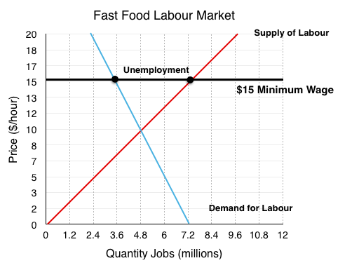
At a wage of $15/hour quantity of labour demanded = 3.6 million, whereas quantity of labour supplied = 7.2 million. The resulting unemployment represents a surplus of workers in the market.
Note that quantity of labour demanded has not fallen by as much as firms are less responsive to the change in wage.
8. What is the deadweight loss from this policy? How does this compare to before?
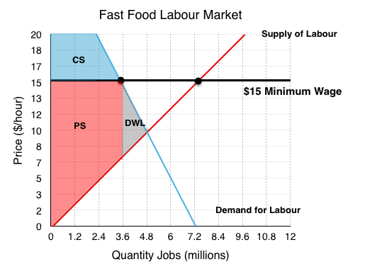
Again we see a deadweight loss as workers lose jobs and firms go out of business. This is equal to the area in grey, labelled DWL.
[latex]\frac{\left(15-7\right)\times \left(4.8-3.6\right)}{2}[/latex] = $4.8 million.
By changing our assumptions of elasticity we see our deadweight loss has fallen from $12 million to $4.8 million. This demonstrates the importance of the assumptions we make, and ensuring that you reveal your assumptions when conducted economic analysis.
9. Comment on how automation effects the elasticity of demand for labour. Would easy access to automation make demand relatively more or less elastic?
All the rhetoric around the increasing accessibility of automation points to the fact that firms demand curves are becoming relatively more elastic. Whereas before there may have been little choice but to have someone at the till, now they can be fairly easily replaced by a machine. This is imporant to recognize when considering the impacts of minimum wage policy, as changing technology can change the assumptions on which we base our models.
