6.3 Understanding Consumer Theory
Learning Objectives
- Understand how the budget line and indifference curve influence a consumers decisions
- Differentiate between the income effect and substitution effect
- Determine whether goods are substitutes/complements and normal/inferior
If we think about the indifference curves in a slightly different way, we see that MRS describes marginal benefit. Since MRS represents the maximum amount of y we are willing to give up in exchange for one unit of x, it also represents how much value our consumer places on x in terms of y.
This means the indifference curve tells us the marginal benefit of good x in terms of good y, and the budget line tells us the marginal cost of good x in terms of good y. As discussed in Topic 1, using marginal analysis, our consumer will continue to purchase more of a good until the marginal benefit is equal to the marginal cost. This means
if MRS > Px/Py, the consumer will consume more x and less y.
If MRS < Px/Py, the consumer will consume less x and more y.
If MRS = Px/Py, the consumer will not change their consumption.
Recall that MRS is the slope of the indifference curve, and Px/Py is the slope of the budget line. This means that if the slope of the indifference curve is steeper than that of the budget line, the consumer will consume more x and less y.
Figure 6.3a shows José’s budget line and possible indifference curves. As Point A, MRS is greater than Px/Py, so José should consume more x and less y to maximize his utility.
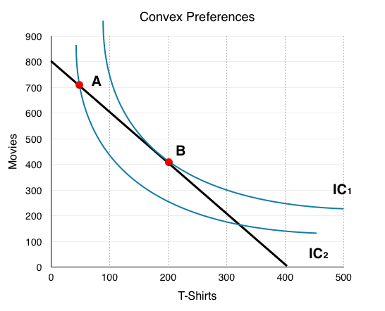
Moving along the budget line (shown in black), we see this action indeed allows José to consume on a higher indifference curve. At point B, MRS = Px/Py, so this is the utility maximizing point, given José’s constraints. Notice that since Point A and Point B are on the same budget line, José could increase utility without a change in expenditures.
In summary, the consumer will consume at the point where the indifference curve and the budget line are tangent, meaning the slopes are equal.
When Prices Changes
We now have all the pieces to develop our model for consumer theory. In Topic 3, we examined the law of demand, which showed that as the price increased our quantity demanded of the good decreased. Now, let’s look at how our consumption choices react to a change in price based on our indifference curve and budget line.
Consider a market with 100 consumers like José, each with budgets of $56 and preferences as illustrated in Figure 6.3b.
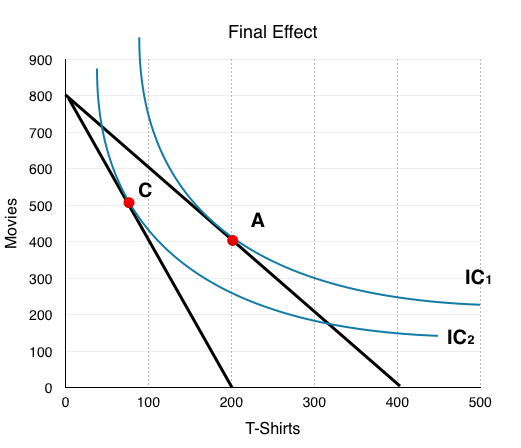
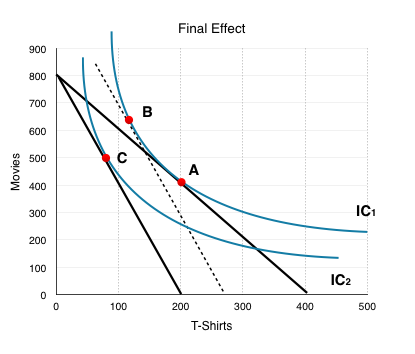
The graph shows the final effect of a price increase on T-shirts. Suppose T-shirts have increased from $14 to $28.
The easiest way to graph a price change is to assume José spends all of his money on T-shirts to see how the intercept will change. Following the price increase, he can only purchase 2 T-shirts. ($56 budget / $28/T-shirt) Because we are imagining a market with 100 consumers like José, all in all, 200 T-shirts will be bought. The price increase causes the budget line to pivot inwards and changes the price ratio from Px/Py = 2 to Px/Py = 4.
Since we know the price of movies has not changed, we know that José can still purchase 8 movies and can show the new graph with our knowledge of these points.
In our example, this causes consumers to change consumption from 200 T-Shirts and 400 Movies (Point A) to around 70 T-Shirts and 500 Movies (Point C). Why is this the case? Can we tell from this graph whether the two goods are compliments or substitutes? Normal or inferior?
To answer these questions, we can decompose the consumer’s response into two parts:
-Draw a BL with the same slope as the new one, but draw it touching the original IC at the point of tangency.
-The movement from the old optimal consumption point to this new tangency point is the SE.
-Draw the final BL associated with the price change.
-The movement from the consumption point on the BL drawn in the SE to the optimal point on the final BL is the IE.
Substitution Effect
Breaking up the effects of a price change involves back-tracking from our final effect. To find the substitution effect, we must do a thought experiment and ask “where would the consumer’s optimal bundle be if they were given back enough money to consume along their original indifference curve?”
At point C in Figure 6.3b, our current budget of $56 brought us to a lower IC. To analyze the SE, we must hold well-being constant and return to our original IC. To do so, we must increase each consumers budget by $23, so we can go back to IC1 at Point B. This is an important step because it shows us how the consumer would respond to the differences in relative prices, holding purchasing power constant. Note the $23 amount is the exact income increase it would take to bring us back tangent with the original indifference curve.
We stated that the substitution effect is purely due to changes in relative prices. To examine its effect, we must compare the two points along our original IC: our first consumption bundle, Point A, and our new consumption bundle, Point B, which represents how our consumer behaves if they feel no poorer. This means the substitution effect is the change from Point A to Point B.
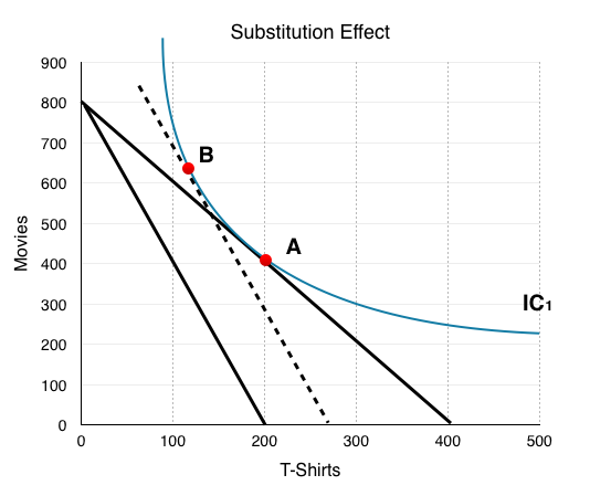
Substitution always has the same effect. People will substitute away from the good which has increased in price because it is relatively more expensive. Since the price ratio is Px/Py, when the price of x increases, Px/Py will be greater. Whereas before Px/Py = MRS, now Px/Py is > MRS. This means the consumer will buy less x and more y until MRS = Px/Py again.
Income Effect
To find our SE we had to hypothetically give the consumer some income to bring them back to their original IC. Though this exercise is simply to show the effect of a price change while holding purchasing power constant, in reality, this sometimes actually happens! Take, for example, a government tax rebate. This is often done to ensure that government increasing prices doesn’t cause consumers to be any worse off than before.
Price increases reduce a consumer’s purchasing power, making them unable to be as happy as they were before. At Point C, although our budget is unchanged at $56, we are not able to stay on IC1 without a large increase in income (back to Point B). The income effect is represented as the movement from Point B, where we are able to consume at the same level of utility as before, to Point C, where the decrease in purchasing power is also represented. This isolates the change to a consumer’s purchasing power, holding relative prices constant.
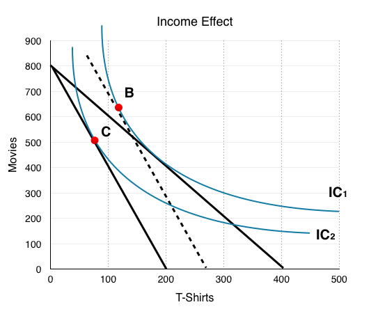
In Figure 6.3d, we see that the individual consumes more T-shirts and movies following an increase in income. In Topic 3, we said that if QD increases when income increases, the good is normal, and if QD decreases when income decreases, it is inferior. This means that both T-shirts and movies are normal goods. This is not always the case. If QD of either good fell after the income increase, it would be inferior.
The Final Effect
To determine the final effect, we need to bring together the income effect and the substitution effect. The SE brought us from Point A to Point B, and the IE from Point B to Point C. We generalize the sum of these effects using X and Y.
Substitution Effect: x decreases, y increases
Income Effect: x decreases, y decreases
With this information, we know the consumer will consume less x, but we are uncertain whether they will consume more or less y. By looking at the movement from Point A to Point C on the graph, we can see the final effect shows the consumer wanting more y and less x.
This provides us with some useful information. Recall in Topic 3, we determined that if two goods are substitutes, when the price of one increases, the demand for the other will increase; whereas if they are complements, when the price of one increases, demand for the other will decrease. In this case, movies and T-shirts are substitutes.
What We Have Learned
Let’s summarize the information we have learned from a simple consumer theory analysis of a price increase. After a price increase in T-shirts from $14 to $28:
- Consumers buy more Movies and Less T-Shirts
- Both Movies and T-Shirts are normal goods (income effect)
- Movies and T-Shirts are substitutes (final effect)
We want to be able to determine these three things for every consumer problem you are given.
Substitutes vs Compliments
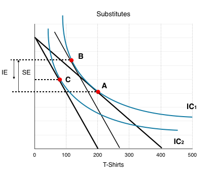
To determine whether two goods are substitutes or complements, we look at the final effect, not the substitution effect. Why call it the substitution effect then? Because to determine the final effect, we must find whether the income effect or the substitution effect is more powerful.
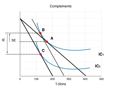
- When the substitution effect overpowers the income effect, the goods are substitutes. (Figure 6.4f)
- When the income effect overpowers the substitution effect, the goods are complements. (Figure 6.4g)
Normal vs Inferior
You should already have a good understanding of how to tell whether a good is normal or inferior based on the income effect. In the example above, we determined that both goods were normal since when we removed the hypothetical income boost, both QD for x and QD for y fell.
Let’s look at a case where prices are decreasing. In Figure 6.4h, the IC and BL are shown for a market where the price of x has fallen, pivoting the budget line from BL1 to BL2. In this case, we must take away the hypothetical income to isolate the SE, bringing us from Point A to Point B. The income effect is simply what happens when we reverse our thought experiment, and either remove the hypothetical income, or in this case, give it back.
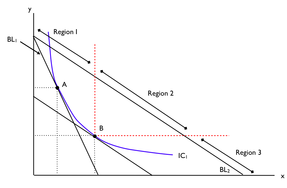
Figure 6.4h presents 3 regions. Whether the goods are inferior or normal will determine where the new IC and Point C end up.
Region 1: QD for X decreases, QD for Y increases
Good X is inferior, Good Y is normal
Region 2: QD for X increases, QD for Y increases
Good X is normal, Good Y is normal
Region 3: QD for X increases, QD for Y decreases
Good X is normal, Good Y is inferior
What if Both Goods Are Inferior?
Both goods cannot be considered inferior in this model, because the model only represents two goods. Whether a good is inferior or normal is relative to other goods. Kraft Dinner is inferior because when I can afford to, I would rather buy Steak. Consider a case where two inferior goods are the only two goods in the market. With your budget, you can either purchase Kraft Dinner or Tomato Soup. Although both could be considered inferior in the regular market, in our market of two goods, when income increases you will either buy more of both, or more of one – never less of both. Remember that economic models are simplifications of reality, because the more variables you include, the more complicated they become.
Conclusion
Consumer theory helps us see how individual consumers behave in a large market. With the model, we can determine whether goods are substitutes or complements, normal or inferior, and use the final effects to see how consumers respond to price changes. In Topic 3, we showed how movements along the demand curve result from changes in prices. In the next section, we will show how this model can be used to derive demand curves.
Glossary
- Income Effect
- The effect of a price change on a consumers purchasing powers, impact depends on whether good is normal or inferior
- Substitution Effect
- the effect of a price change on the relative price of goods, consumers generally substitute away from goods when prices rise
- Tangent
- the slope are equal
Exercises 6.3
1. In the diagram below, a consumer maximizes utility by choosing point A, given BL1.
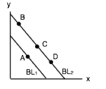
Suppose that both goods x and y are normal and the budget line shifts to BL2. Which of the following could be the new optimal consumption choice?
a) B.
b) C.
c) D.
d) Either B or C or D.
2. Suppose that, given the consumption bundle x = 10 and y = 10, a consumer’s MRS is equal (in absolute value) to 4. The price of x is $1 and the price of good y is $0.25, and the bundle x = 10 and y = 10 uses up all the consumers income. The consumer’s preferences are strictly convex. Which of the following is TRUE?
a) To maximize utility the consumer should but more x and less y.
b) To maximize utility the consumer should buy less x and more y.
c) The bundle x = 10 and and y = 10 maximizes the consumer’s utility.
d) To maximize utility the consumer should buy more of both x and y.
3. The diagram below illustrates the effect of a decrease in the price of good y, for a given consumer.
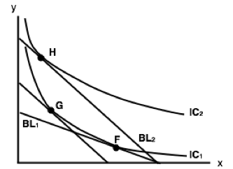
Which of the following statements is TRUE?
a) Goods x and y are substitutes.
b) Goods x and y are complements.
c) Goods x and y are neither substitutes or complements.
d) None of the above statements are true.
4. The diagram below illustrates the effect of a decrease in the price of good y, for a given consumer. Which of the following statements is TRUE?
a) Goods x and y are substitutes.
b) Goods x and y are complements.
c) Goods x and y are neither substitutes or complements.
d) None of the above statements are true.
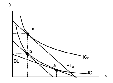
5. Refer to the indifference curve/budget line diagram below.

Suppose that a consumer initially faces budget line BL1, and thus, by choosing consumption point c, is able to achieve the utility level associated with IC1. If px decreases, then the substitution effect is the movement from ______ and the income effect is the movement from ______.
a) a to b; b to c.
b) b to a; a to d.
c) c to d; d to a.
d) d to c; c to b.
6. Refer to the indifference curve/budget line diagram below.
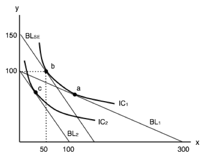
This consumer has $300 in income and initially faces prices of px = $1 and py = $3. Given this, she maximized her utility at point a.
If the price of good x rises to $3, how much additional income would the consumer need, in order to be able to attain her original level of utility given the new prices?
a) There is insufficient information to determine the additional income needed.
b) $450.
c) $300.
d) $150.
7. Refer to the indifference curve/budget line diagram below.
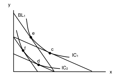
Suppose that a consumer initially faces budget line BL1, and thus is able to achieve the utility level associated with IC1. If py increases, then the substitution effect is the movement from ______ and the income effect is the movement from ______.
a) e to d; d to c.
b) e to c; e to d.
c ) e to c; c to d.
d) e to f; f to d.
8. Suppose that, given the consumption bundle x = 10 and y = 10, a consumer’s MRS is equal (in absolute value) to 0.4. The price of x is $0.50 and the price of good y is $0.75, and the bundle x = 10 and y = 10 uses up all the consumers income. The consumer’s preferences are strictly convex. Which of the following is TRUE?
a) To maximize utility the consumer should buy more x and less y.
b) To maximize utility the consumer should buy less x and more y.
c) The bundle x = 10 and and y = 10 maximizes the consumer’s utility.
d) There is insufficient information to determine what the consumer should do to maximize utility.
