Solution: Case Study – Oil Markets
1. Consider the following producer theory model for a single firm producing oil, and the aggregate supply and demand. What is the firm’s equilibrium price and quantity?
To find price, we look at the aggregate market, where supply = demand. In this case, we find the intersection, labeled E1, occurs at a quantity of 50 million barrels/day and a price of $50/barrel.
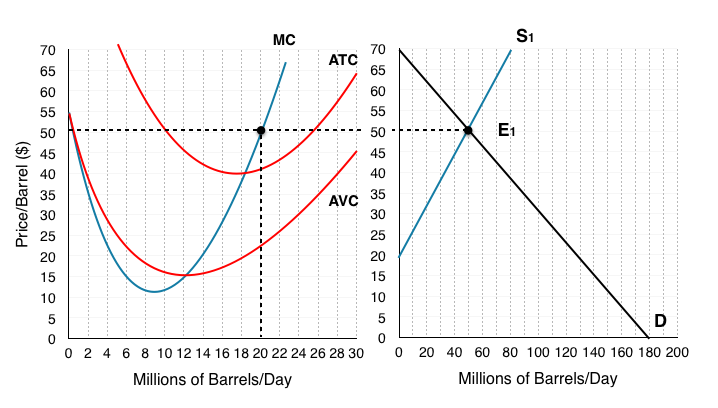
Remember that in order to maximize profits, the firm will produce until MB = MC. Since the market is perfectly competitive, MB = MC when P = MC. This means we must find where our price of $50 intersects our marginal cost curve. Looking at our producer theory diagram, we see that P = MC when the individual firm is producing 20 million barrels/day.
This means our equilibrium price is $50 and our equilibrium quantity is 20 million barrels/day.
2. What is the firm’s profit at this level?
To find firms profits, calculate the area between Price and ATC shown in green. Since price is equal to the marginal revenue for the firm, this green area is the difference between TR (P*Q) and TC (ATC*Q).
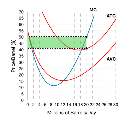
Since MR is $50 and ATC is $41, our firm is making $9 in profit for each barrel of oil. This means that profits are equal to $9 x 20 million barrels, or $180 million.
3. What will occur in the long-run for this market? Show this on the new graph below.
The profits that this firm is making are unsustainable in the long-run, $180 million is attractive to firms in similar industries and will cause entry.
This will cause our supply curve to shift to S2, where price is equal to our firm’s ATC. As long as P > ATC, our firm is making a profit and entry continues to occur. At the price of $40, our firm is making 0 profits and the market is in long-run equilibrium.
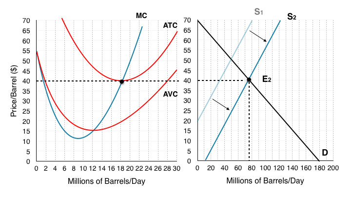
While price fell for a variety of other reasons, the high price certainly incentivized the firms to expand operations, and as we saw in the article, this increase in the production indeed increases supply.
4. Assume the market is at long-run equilibrium. Use the producer theory model from above to show the impact of Iran’s entry, assume this brings the market to a price of $27. What is the new equilibrium price and quantity for the firm?
Iran’s entry will again cause an increase in our supply curve, this time to S3 where our equilibrium (E3) occurs with a price of $27, as specified.
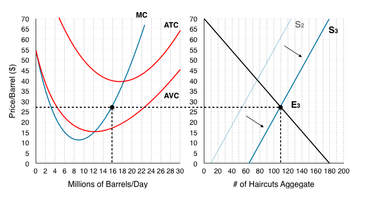
Again, since the market is perfectly competitive, MB = MC when P = MC. Looking where $27 intersects our MC curve, we find that firms will maximize profits by producing 16 million barrels of oil/day.
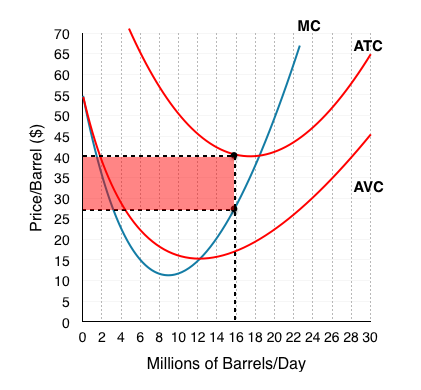
5. What are the firms profits at this price?
In this case, since P < ATC, the firm is making negative profits. In the diagram below, this is indicated by the red area. Since price is equal to the marginal revenue for the firm, this red area is the difference between TR (P*Q) and TC (ATC*Q).
Our total revenue is equal to $27/barrel x 16 million barrels, or $432 million. Total cost is equal to $40/barrel x 16 million barrels, or $640 million. The difference between total revenue and total cost is equal to -$208 million.
6. What does this excerpt suggest about how firms will behave in the short run?
This excerpt hints that the price of $27, while causing losses, is still well above the shut-down price of $15 that would cause firms to shut-down. Since oil production requires considerable capital investment into digging wells, it makes sense that even when in aggregate you are losing money, you will continue to pump oil if you are covering your day-to-day operational costs.
This suggests that the firm will continue to operate in the short-term.
7. Based on the information given about this market, what do you think the time horizon will be for this industries ‘long run’? What will happen in the long run?
Based on the information about the market, you can make a good assumption that the time horizons for an oil firms fixed factor could be well over a few years. Oil wells are projects that take considerable time and resources to develop, and once built are basically used until they run dry. This means that a firm could continue to pump oil from wells for years after knowing that they will not fully recover their fixed costs.
In our model, this means that our supply curve will be slow to adjust to periods of high or low profits. Eventually, the curve will shift back to S2 and profits will return to 0.
8. Comment on the effects of OPEC’s actions on the market.
Normally when prices fall, firms adjust production in the short-run. Comparing the responses in question 3 and 4 you can see that the firm has decreased production from 18 million barrels/day to 16 million barrels to react to the price decrease, an OPEC pact to keep production high would stop that from happening.
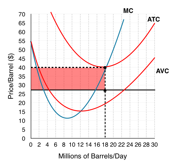
Looking from the firms perspective, we can calculate their new losses and find ($40 – $27)(18) = -$234 million. The pact causes the firm to lose more money because they are operation where MC > MR. While this results in losses, the overproduction can have the effect of keeping out new entrants. In this case, it more likely led to further problems for the industry.
