3.4 Building Supply and Producer Surplus
Learning Objectives
By the end of this section, you will be able to:
- Explain quantity supplied, and the law of supply
- Understand how implicit and explicit costs are used to build a supply curve
- Calculate producer surplus given a marginal cost curve and price
- Explain the divisibility of goods

Now that we have examined demand and its determinants, let’s look at supply. For the most part, the analysis is similar. Let’s start with an example.
The Cupcake Business
When the store “Cupcakes” came to Vancouver in 2002, the cupcake industry was very different than it is today. The start-up was the only one in town and had the ability to set the price as it saw fit. Over 10 years later, the industry has changed. It is now common to see multiple cupcake shops in each city. New York even has a cupcake ATM where customers can buy cupcakes after the store closes. To understand the supply side of the market, let’s look at a cupcake business that operated in a far more competitive market model than the ones mentioned above – Alaythia Cakes. Alaythia Cakes, a small-town business that primarily sold its products at a weekly farmer’s market, was looking to bring its products to the provincial stage with distribution in grocery stores. Compared to the overall market, Alaythia Cakes was a small player, and when negotiating with brands like Save on Foods, Thrifty Foods, and Costco, it found that it had little to no power in negotiating price, since the grocery chains had access to many other cupcakes suppliers (no supplier power).
Opportunity Cost in the Real World
In Topic 2, we looked at the production possibilities of a person on an island, denominating costs in the marginal opportunity cost of an action. Let’s take that island example and apply it to a firm. While Alaythia Cakes was looking to expand, its production possibilities are limited by the owner and the capacity of the staff. The business can choose to produce and sell cookies, cupcakes, or a mix of both. Assume that:
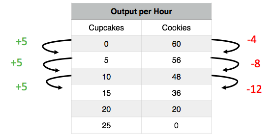
For the first 5 cupcakes, the MC = 0.8 cookies (4 cookies/5 cupcakes)
For the second 5 cupcakes, the MC = 1.6 cookies (8 cookies/5 cupcakes)
For the third 5 cupcakes, the MC = 2.4 cookies (12 cookies/5 cupcakes)
With this information, we can derive the supply curve, but first we need to denominate the marginal cost in the correct medium of exchange – dollars. Let’s assume the current market price for cookies is $0.50 per cookie. Then, for the first 5 cupcakes, implicit costs are $0.50 x 0.8 = $0.4. All we are doing is changing the way we describe cost from ‘cookie terms’ to ‘dollar terms.’ Is this all our costs? Recall in Topic 1 that the opportunity costs of an action include all implicit and explicit costs. In this case, an explicit cost would include the actual cost of flour, eggs, etc. Let’s assume that the explicit costs of a cupcake are $0.5. This means:
MC of 1st 5 cupcakes = $0.5 (explicit) + $0.4 (implicit) = $0.9
MC of 2nd 5 cupcakes = $0.5 (explicit) + $0.8* (implicit) = $1.3
MC of 3rd 5 cupcakes = $0.5 (explicit) + $1.2* (implicit) = $1.7
*the implicit costs were calculated by multiplying the implicit costs denominated in cookies by $0.5.
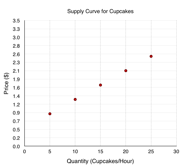
The Supply Curve
To create the supply curve, we need to graphically represent our information. Using price on the y-axis, and quantity on the x-axis, we can plot the marginal cost points to produce Figure 3.4b.
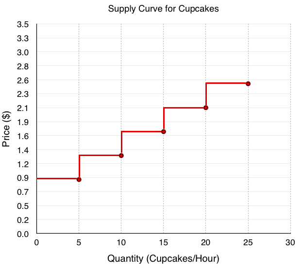
As with demand, we simply join the points in stair-step fashion to create our curve as shown in Figure 3.4c. We can now use our supply curve to examine how our quantity supplied interacts with price, and how this will affect producer surplus.
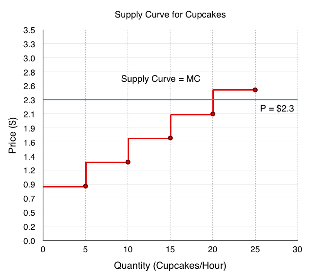
Now, let’s use these tools to determine quantity supplied. Suppose after meeting with the managers of Save-On-Foods, Thrifty Foods, etc. the manager of Alaythia Cakes has determined the best price they can get for the cupcakes is $2.3. By looking at where price intersects the supply curve, we can determine what quantity of cupcakes Alaythia Cakes will supply. Looking at Figure 3.4d, the MC of units 15 to 20 is $2.1, which is less than the price, but the MC of units 20 to 25 is $2.5, which is greater than price. Therefore, Alaythia Cakes will produce 20 cupcakes when the market price is $2.3.
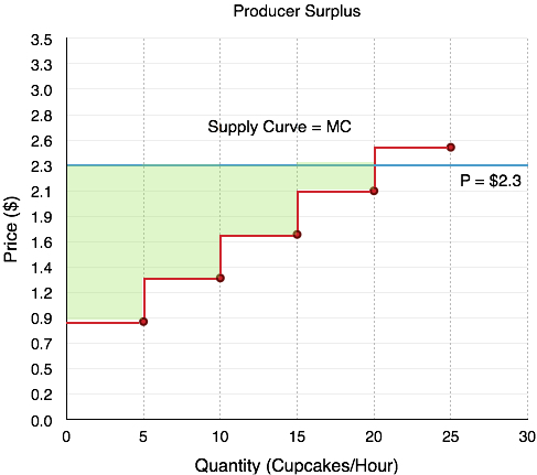
Producer Surplus
Just like consumer surplus, it is important to examine a producer’s net benefit from a certain action. Whereas consumer surplus is the difference between what the consumer is willing to pay and the price they pay, producer surplus is the difference between what the producer is paid (revenue), and the variable cost of production. Our variable costs are represented by our implicit and explicit costs.
How does producer surplus differ from profit?
As we will explore later in the course, there is a key distinction between economic profit and the classic profit calculated in accounting. Economic profit is a firm’s total revenue minus its total costs, including variable, fixed and opportunity costs. Accounting profit, on the other hand, does not include opportunity costs. (In our example, this means implicit costs would be ignored, and we would only look at the $0.5 constant cost per unit).
The main difference between producer surplus and economic profit is fixed costs, the costs of production that don’t vary when the quantity is changed (i.e. rent, equipment purchase). Economic profit subtracts fixed costs, whereas producer surplus does not. We will explore fixed costs in depth soon.
To break down producer surplus, let’s look at the total revenue and total variable costs of producing 20 cupcakes.
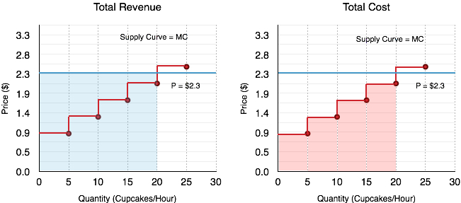
Total Revenue
If the market price of a cupcake is $2.3 and we are producing 20 cupcakes, what is our total revenue? The problem is simple. If you are making $2.3 for every cupcake, and you sell 20, your total revenue will be $46. On the graph, this always corresponds to a rectangle bounded by the price and the quantity supplied (the blue shaded region).
Total Variable Cost
To find total variable cost we need to add the MC at each level, calculating the area under the supply curve (the red shaded region). The calculation of cost for Figure 3.4e is:
Marginal cost of the 1st 5 cupcakes = $0.9 x 5 cupcakes = $4.5
Marginal cost of the 2nd 5 cupcakes = $1.3 x 5 cupcakes = $6.5
Marginal cost of the 3rd 5 cupcakes = $1.7 x 5 cupcakes = $8.5
Marginal cost of the 4th 5 cupcakes = $2.1 x 5 cupcakes = $10.5
Total variable costs ($4.5 + $6.5 + $8.5 + $10.5) = $30
Producer Surplus
Bringing all this information together we can calculate producer surplus. Since Total Revenue – Total Variable Costs = Producer Surplus (PS), our PS is equal to $46 – $30 = $16. This corresponds to the area between the price producers receive, and their costs, shown in green in Figure 3.4f.
Producer Surplus with Changing Prices
Determining producer surplus with changing prices closely mirrors that of consumer surplus during changing prices, but in order to get comfortable with the terminology, we will analyze the effects separately.
Suppose the manager of Alaythia Cakes had been happily selling cupcakes to the grocery stores at $2.3, but one morning, all the grocery stores told him that the best price they could give him was now $1.4/cupcake. According to the law of supply, we know this decrease in price will cause a decrease in quantity supplied, but how does our producer surplus change? Calculating the change in the green area in Figure 3.4g, we see that producer surplus falls from $16 to $3. This change is due to two factors. Firstly, at the lower price, the business can no longer sustain production of 20 units as MC > P, so it decreases the quantity supplied to 10 units. This causes the firm to lose the $4 of producer surplus it was receiving from selling units 10-20. Second, the firm is now receiving a lower price for the units it continues to produce, a total of $0.9 fewer dollars on 10 units, resulting in the other $9 decrease in producer surplus.
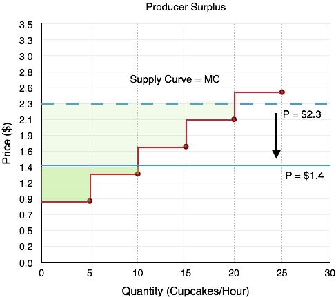
In short, when there is a fall in price, producer surplus decreases for two reasons:
- The quantity produced decreases
- The price the producer receives for the remaining goods decreases
Completing the Supply Curve
The last step we have in the derivation of supply is recognizing that there is divisibility of goods. In the stair-step example, we are implicitly assuming that we can only trade cupcakes and cookies in 5 cupcake increments. Of course, this is not actually the case. The more divisibility we introduce, the more our supply curve smooths out until it is a straight line.
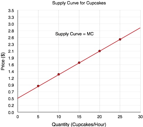
In our analysis of the interaction between supply and demand (equilibrium), we will continue to use smoothed out supply and demand curves. Not only are these curves based on more realistic assumptions, they also lead to greater versatility for mathematical analysis.
Summary
In this section, we examined the market from the eyes of the producer and introduced producer surplus to explain how a firm reacts to price changes. We showed that a change in producer surplus is due to a change in quantity and a change in price, and learned that most supply curves are smoothed out by the divisibility of goods. Before we look at the equilibrium, let us finish the supply picture by looking at some other determinants of supply.
Glossary
- Excess Supply
- at the existing price, quantity supplied exceeds the quantity demanded; also called a surplus
- Law of Supply
- the common relationship that a higher price leads to a greater quantity supplied and a lower price leads to a lower quantity supplied, while all other variables are held constant
- Marginal Cost
- the additional cost that a firm incurs for producing an additional unit of a good or service.
- Producer Surplus
- the difference between a producers costs, and the price they are paid
- Quantity Supplied
- the total number of units of a good or service producers are willing to sell at a given price
- Supply Curve
- a line that shows the relationship between price and quantity supplied on a graph, with quantity supplied on the horizontal axis and price on the vertical axis
- Supply Schedule
- a table that shows a range of prices for a good or service and the quantity supplied at each price
- Supply
- the relationship between price and the quantity supplied of a certain good or service
Exercises 3.4
1. An individual producer’s supply curve for a good is derived from:
a) The preferences of consumers of that good.
b) The income of consumers of that good.
c) The marginal cost of producing that good.
d) All of the above.
The following TWO questions refer to the supply curve diagram below.
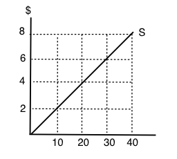
2. If price is $8 per unit, quantity supplied will equal:
a) 10.
b) 20.
c) 30.
d) 40.
3. If quantity supplied increases from 10 to 20 units, the producer’s total costs will increase by:
a) $20.
b) $30.
c) $40.
d) $80.
4. Which of the following statements about supply curves is TRUE?
a) The “law of supply” states that as price rises, quantity supplied also rises.
b) If the marginal cost of producing a good is higher at high levels of output than at low levels of output, then the supply curve for that good is upward sloping.
c) Both a) and b) are true.
d) Neither a) nor b) are true.
5. When deciding how much of a particular good to produce, a producer should:
a) Keep producing more units until the total benefits equal the total costs.
b) Always produce an additional unit if price is greater than marginal cost.
c) Never produce an additional unit if its marginal cost is higher than the marginal cost of previously produced units.
d) Always produce at additional unit if price is greater than zero.
The following TWO questions refer to the diagram below, which illustrates a supply curve.
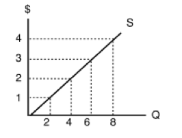
6. In order for quantity supplied to equal 6 units, the price per unit must be:
a) $1.
b) $2.
c) $3.
d) $4.
7. If the price of this good is $4 per unit, then what does producer surplus equal?
a) $32.
b) $24.
c) $16.
d) $12.
8. The diagram below illustrates a supply curve.
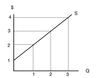
If the price of this good is $2 per unit, then what will be the quantity supplied?
a) 0.
b) 1.
c) 2.
d) 3.
9. Sarah is selling her used truck. The minimum amount she needs to be paid for the truck is $5,000. She advertises the truck on usedvictoria.com for $8,000, and eventually sells the truck for $6,000. Her producer surplus is equal to _____.
a) $1,000.
b) $2,000.
c) $3,000.
d) $6,000.
