5.1 Externalities
Learning Objectives
By the end of this section, you will be able to:
- Explain and give examples of positive and negative externalities.
- Identify equilibrium price and quantity.
In Topics 3 and 4 we introduced the concept of a market. In particular, we closely examined perfectly competitive markets. We observed how producers and consumers of a good interacted to reach equilibrium. We also demonstrated that any policy that was introduced (i.e. quota, price control, tax, etc.) moved the market away from the surplus maximizing equilibrium and created a deadweight loss.
Our assumption throughout this analysis, however, was that there was no third party impacted by the interaction of producers and consumers. We can now add the concept of Externalities to our supply and demand model to account for the impact of market interactions on external agents. We will find that the equilibrium that is optimal for consumers and producers of the good may be sub-optimal for society. We will learn that the all-regulation-is-bad-regulation conclusion from earlier is not always the case – in many situations, we can improve societal outcomes with policy. Before we get to this conclusion, let’s first unpack this concept of externalities.
Externalities
Enriching Our Model
As discussed earlier, we have previously modelled private markets. Thus, the terminology we used in that analysis applies to private markets. The terms consumer surplus, producer surplus, market surplus, and the market equilibrium (note that this will be referred to interchangeably in this chapter as the unregulated market equilibrium) derive their meaning from an analysis of private markets and need to be adapted in a discussion where external costs or external benefits are present.
For the purpose of this analysis, the following terminology will be used:
- Our topic three demand curve is equivalent to the marginal private benefit curve.
- Our topic three supply curve is equivalent to the marginal private cost curve.
We now want to develop a model that accounts for positive and negative externalities. To do so, we must consider the external costs and benefits. External costs and benefits occur when producing or consuming a good or service imposes a cost/benefit upon a third party. When we account for external costs and benefits, the following definitions apply:
- When we add external benefits to private benefits, we create a marginal social benefit curve. In the presence of a positive externality (with a constant marginal external benefit), this curve lies above the demand curve at all quantities.
- When we add external costs to private costs, we create a marginal social cost curve. In the presence of a negative externality (with a constant marginal external cost), this curve lies above the supply curve at all quantities.
When we were considering private markets, our objective was to maximize market surplus or total private benefits minus total private costs. Our new objective considering all impacted agents in society is to maximize social surplus or total social benefits minus total social costs.
Recall that in this course, our diagrams reflect “marginal” quantities. Notice that some of the definitions require you to use “total” quantities. Remember that to derive a “total” from a “marginal,” take the area underneath the marginal up to a quantity of interest. This quantity is often the equilibrium.
A Negative Externality
Much of the work we will do is with negative externalities. As we will see in the next section, pollution is modelled as a negative externality. Economists illustrate the social costs of production with a demand and supply diagram. For example, consider Figure 5.1a, which shows a negative externality. Notice that there are external costs but no external benefits. Graphically, this means that the marginal social cost (MSC) curve lies above the marginal private cost (MPC) curve by an amount equal to the marginal external cost (MEC) and the marginal private benefit (MPB) and marginal social benefit (MSB) are equivalent.
Let’s undergo an analysis of this diagram to understand how we need to shift our thinking from Topic 3 and 4 to Topic 5.
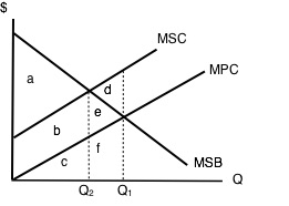
Let’s first pretend we know nothing about externalities and ignore MSC. Market equilibrium in this diagram occurs at the intersection of supply and demand, or the intersection of MPC and MSB (which is equivalent to MPB). This occurs at Q1. Now we know that total private benefits at the market equilibrium are equal to a+b+c+e+f and we know that total private cost at the market equilibrium equals c+f.
The market surplus at Q1 is equal to (total private benefits – total private costs), in this case, a+b+e. [(a+b+c+e+f) – (c+f)].
Now, let’s introduce some of the concepts we’ve learned in this section to our analysis. To get a true picture of surplus, we need to account for the external cost of production. Recall that social surplus is the difference between total social benefits and total social cost. Social surplus is sometimes referred to as aggregate net benefits. Since there is no positive externality, social benefit and private benefit are equal. Thus, as before, it is equal to a+b+c+e+f.
Total social cost at the market equilibrium is equal to b+c+d+e+f, and includes all the areas under our MSC curve up to our quantity. Notice that this is larger than total private cost by b+e+d. This should make sense as we are analyzing a negative externality where, by definition, the private cost to producers is smaller than the social cost of their actions. The difference is these two values is equal to the external costs.
The social surplus at Q1 is equal to total social benefits – total social costs. In this case, a-d. [(a+b+c+e+f) – (b+c+d+e+f)].
In Topic 3 and 4, we saw that the market equilibrium quantity maximized market surplus and that any move away from this quantity caused a deadweight loss. Let’s see if this conclusion holds when we introduce externalities.
Consider our diagram of a negative externality again. Let’s pick an arbitrary value that is less than Q1 (our optimal market equilibrium). Consider Q2.
If we were to calculate market surplus, we would find that market surplus is lower at Q2 than at Q1 by triangle e.
The market surplus at Q2 is equal to area a+b. [(a+b+c) – (c)].
What about social surplus? Total social benefit at Q2 is equal to a+b+c. Total social cost at Q2 is equal to b+c.
The social surplus at Q2 is equal to area a [(a+b+c) – (b+c)].
This result is interesting. By moving to a quantity lower than our optimal market equilibrium, we raised social surplus. Compared to Q1 we have increased our social surplus by area d. This means that d was a deadweight loss from being at the optimal market level of production. That is to say, the optimal market level of production was inefficient for society. By leaving the market unregulated and letting the interaction of producers and consumers set quantity and price, society as a whole is worse off than if quantity had been restricted by policy for example. This means that there is an opportunity for government intervention to make society better off.
Why is this the case? Well, at Q1, we see that our MSC is greater than our MSB. Using marginal analysis, we know that when MC > MB, we need to reduce our quantity to maximize surplus.
How do you know which quantity maximizes surplus?
- When looking for the market equilibrium (sometimes called the unregulated market equilibrium), we want to select the quantity where demand = supply or where marginal private benefit = marginal private cost. Diagrammatically, this will happen where MPB intersects MPC. The quantity where this occurs will always maximize market surplus.
- When looking for the social surplus maximizing equilibrium, we want to select the quantity where marginal social benefit = marginal social cost. Diagrammatically, this will happen where MSB intersects MSC. The quantity where this occurs will always maximize social surplus.
Pareto Improvements and Potential Pareto Improvement
At this point, there may be some confusion around our analysis. The market (or private agents) were worse off in the move from Q1 to Q2, but society was made better off. How is this possible? What criteria are we using to judge if our action to restrict quantity is appropriate? Recall our definition of efficiency from earlier topics. We defined Pareto-efficiency as an outcome where no one can be made better off without making someone worse off. As it turns out, we need two additional definitions to fully understand the movement from an inefficient to an efficient allocation.
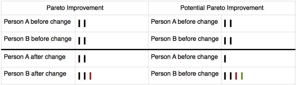
The first term we need to become familiar with is a Pareto Improvement. A Pareto Improvement is a change such that someone is made better off without making anybody worse off. Consider the following example. You only like peanut butter and jelly sandwiches, but your mom has packed you a PB & J and a Nutella sandwich. Your friend has no sandwiches in their lunch bag but loves sandwiches. Since you do not value Nutella sandwiches, if you give your friend your Nutella sandwich, you would make them better off without making yourself worse off (remember, you don’t place any value on Nutella sandwiches). This scenario describes a Pareto Improvement.
The second term we need to introduce is a Potential Pareto Improvement. The definition of a Potential Pareto Improvement has three parts:
- As opposed to a Pareto Improvement, a Potential Pareto Improvement may have people who gain and people who lose.
- The individuals who gain from the change gain by enough that in theory some of their gains could be taken to compensate those who lose such that we again have a scenario where people are made better off without making anybody worse off.
- The compensation just needs to be possible. It does not have to occur for a change to be a Potential Pareto Improvement.
Note that all Pareto Improvements are necessarily Potential Pareto Improvements but not all Potential Pareto Improvements are necessarily Pareto Improvements.
It should also be noted that if social surplus increased, at the very least Potential Pareto Improvement occurred. Pareto Improvements almost never exists and thus do not form that basis of decision making in the policy process. More often than not the choices we make are based on Potential Pareto Improvements.
Let’s illustrate a Potential Pareto Improvement and compare it to a Pareto improvement with the following illustration.
Potential Pareto Improvements to Externalities
Private Agents
Let’s first consider private market participants. In the move from Q1 to Q2, private agents reduce their costs by f (they are producing less so costs should be less; f is the area underneath the marginal private cost curve between Q2 and Q1) but also decrease their benefit by e+f (the area under the marginal private benefit curve between the two quantities of interest). On balance, they are worse off by e. when they move from Q1 to Q2.
External Agents
In the move from Q1 to Q2, the external cost imposed declines by d+e, meaning they are better off by d+e. Remember when looking for external costs, we are looking under the MSC curve but above the MPC curve.
To determine whether this is a Potential Pareto Improvement, we need to find out whether the gains from the winners exceed the losses to others. In our example, the gain by external agents is indeed larger than the loss to private agents (d+e > e). Therefore, in theory, we could take e from the external agents and give it to the private agents and make them equally as well off as they were at the market equilibrium. External agents would still be better off by d. Thus, a Potential Pareto Improvement has been realized.
This resolves the tension we brought up at the beginning of this section and explains how we can increase social surplus by changing the quantity from the market equilibrium.
Positive Externalities
As we mentioned previously, a positive externality occurs when the market interaction of others presents a benefit to non-market participants. The analysis of positive externalities is almost identical to negative externalities. The difference is that instead of the market equilibrium quantity being too much, the market will generate too little of Q. Let’s look at an example. Consider the following diagram of a market where a positive externality is present.
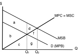
Notice first that MPC curve is the same as MSC curve because there are no external costs. Second, the MSB curve lies above the MPB curve at all quantities because each unit of private consumption generates a spill-over benefit to non-market participants. The area in between MSB and MPB is the external benefit. Remember that MPB + MEB = MSB.
Let’s briefly explore this diagram as we did for negative externalities. The market equilibrium occurs where MPB = MPC. That occurs at Q1.
The market surplus at Q1 is equal to total private benefits – total private costs, in this case b. [(b+c) – (c)].
The social surplus at Q1 is equal to total social benefits – total social costs, in this case a+b. [(a+b+c) – (c)].
As before, suppose we increased the quantity in this market to Q2.
The market surplus at Q2 is equal to b-f. [(b+c+g) – (c+f+g)].
The social surplus at Q2 is equal to a+b+d. [(a+b+c+d+f+g) – (c+f+g)].
Note that social surplus has increased despite the fact that market participants are worse off. Thus, a Potential Pareto Improvement must have occurred. We can see this is the case by noticing that d+f is the amount that non-market participants gained by the increase in production and that f is the loss to market participants from excess production. In theory, we could take f from the external agents and give it to the market participants so they would be indifferent to the situation before and after the change. Thus, we know that d is the deadweight loss in the presence of a positive externality, due to under production.
Okay, but what’s an example of a Positive and a Negative Externality?
As an example of a Negative Externality: Suppose a banana farmer uses pesticides on their crop and some of this pesticide runs off into a nearby stream that is the primary water supply of a downstream community. The farmer and the banana consumers do not account for the negative impact the operations have on the stream. In other words, there is a spillover cost inherent to this market interaction.
As an example of a Positive Externality: suppose a bee keeper’s hives are located near another farmer’s orchard. The bees fly to the orchard and pollinate the crop resulting in a spillover benefit for the orchard farmer.
Key Concepts and Summary
Economic production can cause environmental damage. This trade-off arises for all countries, whether they be high-income or low-income, and whether their economies are market-oriented or command-oriented.
An externality occurs when an exchange between a buyer and seller has an impact on a third party who is not part of the exchange.
An externality can have a negative or positive impact on the third party. If those parties imposing a negative externality on others had to take the broader social cost of their behaviour into account, they would have an incentive to reduce the production of whatever is causing the negative externality.
In the case of a positive externality, the third party is obtaining benefits from the exchange between a buyer and a seller, but they are not paying for these benefits. If this is the case, markets tend to under-produce output because suppliers do not consider the additional benefits to others. If the parties that are creating benefits for others can somehow be compensated for these external benefits, they would have an incentive to increase production.
Glossary
- External Benefits
- additional benefits reaped by third parties outside the production process when a unit of output is produced
- External Cost
- additional costs incurred by third parties outside the production process when a unit of output is produced
- Externality
- a market exchange that affects a third party who is outside or “external” to the exchange; sometimes called a “spillover”
- Market Failure
- When the market on its own does not allocate resources efficiently in a way that balances social costs and benefits; externalities are one example of a market failure
- Negative Externality
- a situation where a third party, outside the transaction, suffers from a market transaction by others
- Positive Externality
- a situation where a third party, outside the transaction, benefits from a market transaction by others
- Private Market
- a market that only considers consumers, producers and the government, doesn’t include external agents
- Social Costs
- costs that include both the private costs incurred by firms and also additional costs incurred by third parties outside the production process, like costs of pollution
- Spillover
- see externality
Exercises 5.1
1. Which of the following statements about negative externalities is/are TRUE?
I. At the social-surplus maximizing level of output, external costs equal zero.
II. At the unregulated competitive equilibrium, marginal social cost is greater than marginal social benefit.
III. At any output level, social costs are greater than private (market) costs.
a) I, II, and III.
b) II only.
c) III only.
d) II and III.
2. Which of the following statements about external costs is TRUE?
a) Economics uses the term “external cost” to describe a spillover effect from market activity that is too small to matter to society.
b) Economics ignores the environmental impact of market activities by calling such impact an “external cost.”
c) Economics does not provide guidance for environmental policy since its treats any environmental cost as an “external cost”.
d) None of the above statements are true.
3. If a competitive market is characterized by a negative externality, then which of the following statements is true?
a) Social surplus is greater than market surplus.
b) Social surplus is less than market surplus.
c) Social surplus is equal to market surplus.
d) Social surplus may be greater than or less than market surplus, depending on the size of the externality.
The following TWO questions refer to the diagram below, which illustrates the market for a good whose production results in a negative externality.
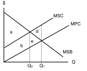
4. If there is no regulation in place to correct the externality, which area represents MARKET surplus?
a) a.
b) a – d.
c) a + b.
d) a + b + e.
5. If there is no regulation in place to correct the externality, which area represents SOCIAL surplus?
a) a.
b) a – d.
c) a + b.
d) a + b + e.
6. Suppose that each kilowatt-hour (kwh) of electricity produced using natural gas results in 0.2kgs of carbon dioxide emissions. If each ton of carbon dioxide emissions results in environmental costs of $360, then the marginal external cost per kwh of electricity produced is equal to (0.2kg is equal to about 0.000220462 tons):
a) 10 cents.
b) 8 cents.
c) 4 cents.
d) 2 cents.
The following THREE question refer to the diagram below, which illustrates the marginal private cost, marginal social cost, and marginal social benefits for a goods whose production results in a negative externality.
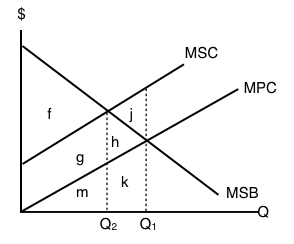
7. Which are represents the deadweight loss due to the externality?
a) j.
b) h.
c) h+j.
d) There is no deadweight loss.
8. Which are represents external costs at the unregulated competitive equilibrium?
a) g + h + j + m + k.
b) g + h + j.
c) g + m.
d) g.
9. Which are represents social surplus at the unregulated competitive equilibrium?
a) f – j.
b) f.
c) f + g + h.
d) f + g + h – j.
Save
Save
