3.2 Building Demand and Consumer Surplus
Learning Objectives
By the end of this section, you will be able to:
- Explain quantity demanded, and the law of demand
- Identify a demand curve
- Calculate consumer surplus given a Marginal Benefit curve and price
The Law of Demand
Economists use the term demand to refer to the amount of some good or service consumers are willing and able to purchase at each price. Demand is based on needs and wants, and while consumers can differentiate between a need and a want, from an economist’s perspective, they are the same thing. Demand is also based on ability to pay. If you cannot pay for it, you have no effective demand. This concept of a consumer’s willingness to pay (WTP) serves as a starting point for the demand curve. A consumer’s Willingness to Pay is equal to that consumer’s Marginal Benefit (MB). This is useful information if we want to use Marginal Analysis.
As we learned in Topic 1, Marginal Analysis or “thinking on the margin” is how consumers decide whether or not to buy an additional unit. It is the process of considering the additional benefits and costs of an activity to make a decision. Therefore, when we say a consumer is willing to pay x dollars for another good, we are stating that the consumer believes they will receive x amount of benefit. As long as the consumer’s marginal benefit is greater than their marginal cost, they will purchase the good. Therefore, the maximum amount a consumer is willing to pay is equal to their marginal benefit.
What a buyer pays for a unit of a good or service is called price. The total number of units purchased at that price is called the quantity demanded. A rise in price of a good or service will almost always decrease the quantity demanded of that good or service. Conversely, a fall in price will increase the quantity demanded. Economists call this inverse relationship between price and quantity demanded the law of demand. The law of demand assumes that all other variables that affect demand (to be explained in Topic 4) are held constant.

Let’s look at these concepts in more detail with an example. Assume that your car holds 50L of gas and that at the average price of gas you would generally use about a tank of gas each month. This amount allows you to comfortably drive to school and back, run errands, and use the car on weekends for trips. As discussed above, this usage will change as price changes.
Demand Schedules and Curves
As a student on a tight budget, the price of gas will have a large influence on the amount you drive. When the price of gasoline goes up, you will look for ways to reduce your driving by combining errands, commuting by carpool or transit, biking and walking more, and driving less on weekends and holidays. So, what would happen if the price of gas was $3.5/litre? Though you would likely be outraged that prices had risen so high, would you stop driving altogether? Perhaps, but perhaps not. Assuming there are some cases where your marginal benefit for driving is so high that you are willing to pay this high premium, we can estimate that you might use about one tank over the semester. This is about one quarter of the driving you are used to. This shows that for the first 50L of gas you consume, you are willing to pay a high price, in this case $3.5/L.
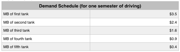
If, from the high price of $3.5, the price falls to $2.4, you will drive more. At this price you may use 100L of gas, or about two tanks, over the course of a semester. Using this we can make a demand schedule, as shown in Figure 3.2a, for a typical student. This illustrates the law of demand. For the first tank of gas you were willing to pay a high price of $3.5/L, but for the second tank you were only willing to pay $2.4/L. As price falls, the quantity you demand increases.
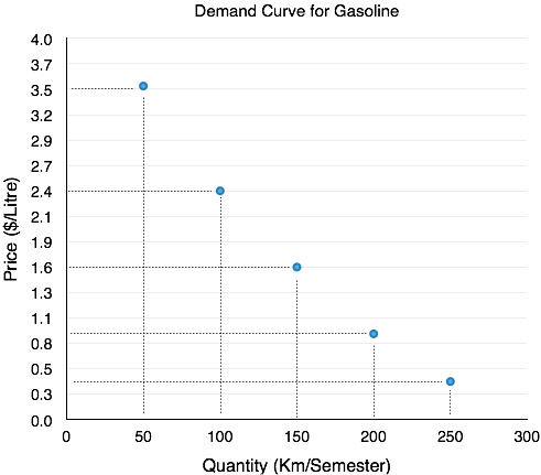
This analysis can be continued for the third, fourth, and fifth tanks of gas. To create a more visual representation, we can plot the quantities of gas a student is willing to buy at varying prices on a graph as shown in Figure 3.2b. Once again, we see that as the price falls, quantity demanded increases.
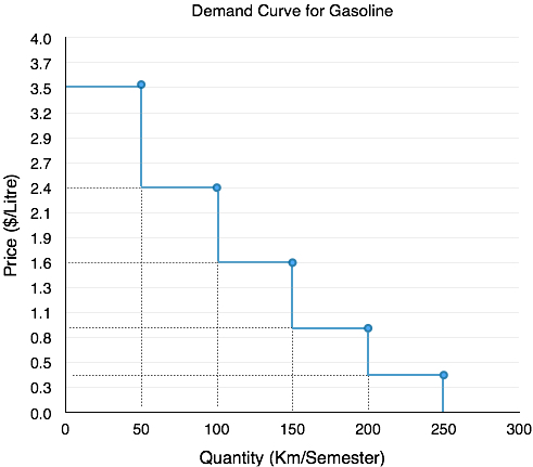
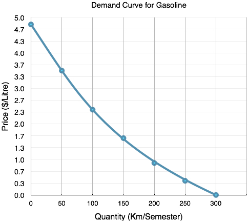
If we join the points together as in Figure 3.2c, we produce a demand curve – a graphical representation of our demand schedule. This is the same as a Marginal Benefit Curve, as it shows the consumers marginal benefit at a given quantity.
The Ceteris Paribus Assumption
In section 3.1, we mentioned that we hold certain variables constant to analyze the ones that are most important. In the case of the demand curve (and the supply curve, as we will soon see), we are examining a relationship between two, and only two, variables: quantity on the horizontal axis and price on the vertical axis. The assumption behind a demand or supply curve is that no economic factors other than the product’s price are changing. Economists call this assumption ceteris paribus, a Latin phrase meaning “other things being equal.” Any given demand or supply curve is based on the ceteris paribus assumption that all else is held equal. If all else is not held equal, then the laws of supply and demand will not necessarily hold.
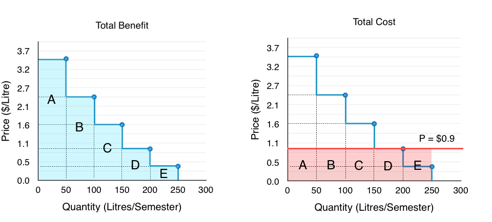
With the information about our demand curve and with the ceteris paribus assumption, we can determine what quantity our student will consume at a given price. So, what if our price is $0.9? This is fairly close to what you would expect to pay for gas in the current market. Alas, by examining the demand curve in Figure 3.2d, we see what we had discussed earlier. The student will travel about 200 km per semester, using about a tank of gas each month. We determine this by looking at where price is equal to the student’s marginal benefit, or where the price line intersects the demand curve.
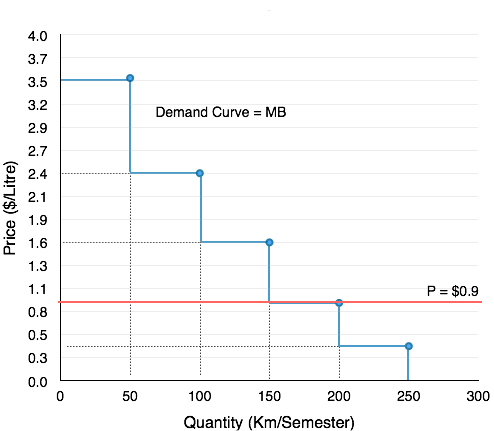
In Topic 1, we determined that a consumer will purchase something as long as MB > MC. Since the price of gas is constant in this example, the student’s marginal cost is constant as well. Why does the student not consume 50L of gas? At 50L, the student’s MB is $3.5, which is greater than the MC of $0.9. Likewise, the MB at 100 and 150L is also greater. At 200L, the MB is equal to the marginal cost of $0.9, so the student will purchase 200L. Any more and MB will fall below MC, meaning the cost of the action outweighs the benefits.
Consumer Surplus
Notice that for the first 150L of gas purchased, the student’s MB is greater than his MC. In Topic 1, we discussed that this difference is equal to the marginal net benefit. By examining the marginal net benefit at each level of consumption, we can measure a consumer’s total net benefit from their purchase, or their consumer surplus. Consumer surplus is the difference between the consumer’s willingness to pay and the amount they actually pay for a given quantity, or the total benefits minus the total costs of consumption.
Looking at Figure 3.2e, we can see that the benefit from each 50L increase is diminishing. For the first 50L, where our marginal benefit from consumption is $3.5/L, our total benefit is equal to area A, or $175, whereas our next 50L only give us a additional benefit of area B, or $120. Regardless, these 50L still increase our total benefit from $175 to $295. Our total cost from the first 50L is $0.9/L or $45
Notice that for the first 150L of gas purchased, the student’s MB is greater than his MC. In Topic 1, we discussed that this difference is equal to the student’s marginal net benefit. By examining the marginal net benefit at each level of consumption, we can measure a consumer’s total net benefit from their purchase, or their consumer surplus. Consumer surplus is the difference between the consumer’s willingness to pay and the amount they actually pay for a given quantity, or the total benefits minus the total costs of consumption.
We can break down how this corresponds to consumer surplus with marginal analysis. For the first 50 units of production, with total benefit of $175 and total cost of $45, our consumer surplus is equal to $130. We continue this analysis in Figure 3.6f. As long as our MB is greater than our MC, consumer surplus will continue to increase.
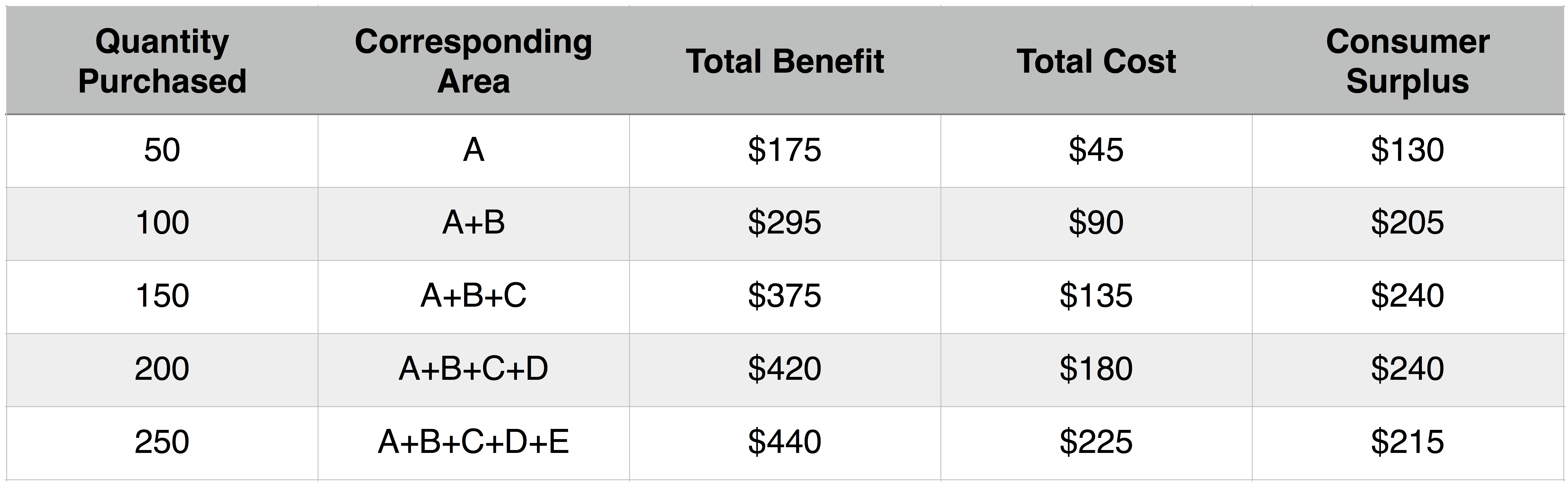
Take special note of total benefits and total costs at the consumption level of 250. Recall that we determined the optimal level of production was when MB = MC. With our price of $0.9, this occurred when quantity demanded was equal to 200L. Students often get confused when looking at the table above and point out that at 250L, total benefits are greater than total costs, and reason that the consumer should continue to consume beyond 200L, but remember, it is not the total benefits and costs that matter in marginal analysis. For example, if you were willing to pay $1 for a Coke but it costs $3, it doesn’t matter how many Cokes you purchased previously, or the benefit or costs of those former Cokes. All that matters are the costs and benefits for the next unit of consumption. This is the heart of marginal analysis.
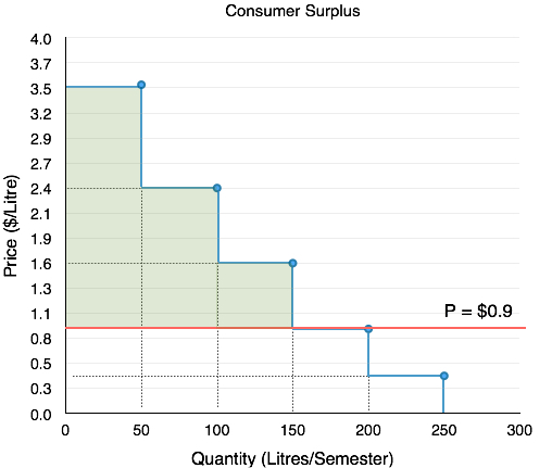
Bringing the marginal analysis together, we can look holistically at consumer surplus. Recall that consumer surplus is just the difference between the consumers willingness to pay (the blue line) and the cost to the consumer (the red line). By calculating this area (shown shaded in green in Figure 3.2g) we can easily find consumer surplus without having to look separately at Total Benefits and Total Costs.
Consumer Surplus with Changing Prices
We have now examined the consumer surplus when price is $0.9/L, but what if our price changes? Suppose that price suddenly rises to $2.4/L. By the law of demand, we have established that this increase in price will cause a decrease in quantity demanded, but it is also important to explore how consumer surplus changes. Consumer surplus can be used to analyze changes in consumer well-being as market conditions change, making it a useful tool to analyze how society is impacted.
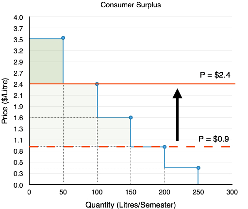
In Figure 3.2h, we see that consumer surplus decreases from $240 to $55. This fall is caused by two factors. First, the student is buying less gas. As discussed before, when price is $2.4/L, the student will combine errands, etc. to decrease the amount they drive. Second, the gas they continue to buy (100L) is now more expensive than before. We can summarize these two changes easily. When prices increase, consumer surplus decreases because:
- The quantity that the consumer consumes decreases.
- The price of the goods the consumer continues to buy increases.
Completing the Demand Curve
The last component of the demand curve to discuss is the divisibility of goods. In our example above, how would quantity demanded change if price increased from $0.9/L to $1.0/L? In our example, it falls from 200L demanded to 150L demanded! What about a price increase from $0.9/L to $1.6/L? Again our quantity demanded falls from 200L to 150L. Does this mean the price increase from $1.0/L to $1.6/L means nothing? This problem is due to the fact that we only examined five possible points on our curve. In reality, the demand curve has an infinite number of relationships between price and quantity
If we were to plot the quantity demanded for every possible price of gasoline, we find a smoothed-out curve like the one shown in Figure 3.2i. When we do this, we fin the quantity demanded for $1.0/L of gas is different than the quantity demanded for $0.99/L of gas. In reality, the average consumer may not change his or her consumption of gas in response to such a minor price change, and may have a demand curve that looks more like the staircases presented earlier, but when you bring together the millions of Canadian gas purchasers with varying willingness to pay, different reactions to prices changes, etc. the divisibility of goods becomes more plausible.
Summary
In this section, we examined the market from the eyes of the consumer and introduced consumer surplus to explain how a consumer reacts to price changes. In section 3.4, we will examine the market from the eyes of the producer and introduce the concept of producer surplus. With a strong understanding of consumer and producer surplus, we can examine the impact that changes in the market have on society. Before we get there, we must examine the other determinants of demand that can impact our demand curve.
Glossary
- Ceteris Paribus
- all else equal
- Consumer Surplus
- the difference between a consumer’s willingness to pay, and the price they actually pay
- Demand Curve
- a graphic representation of the relationship between price and quantity demanded of a certain good or service, with quantity on the horizontal axis and the price on the vertical axis
- Demand Schedule
- a table that shows a range of prices for a certain good or service and the quantity demanded at each price
- Demand
- the relationship between price and the quantity demanded of a certain good or service
- Law of Demand
- the common relationship that a higher price leads to a lower quantity demanded of a certain good or service and a lower price leads to a higher quantity demanded, while all other variables are held constant
- Marginal Benefit (MB)
- the additional satisfaction or utility that a person receives from consuming an additional unit of a good or service, equal to WTP
- Marginal Analysis
- an examination of the additional benefits of an activity compared to the additional costs incurred by that same activity, used as a decision-making tool
- Price
- what a buyer pays for a unit of the specific good or service
- Quantity Demanded
- the total number of units of a good or service consumers are willing to purchase at a given price
- Willingness to Pay (WTP)
- the largest sum of money an individual is willing to give up to receive a product or service
Exercises 3.2
1. A buyer has purchased three units of good X. The marginal benefit of the fourth unit of X exceeds the marginal cost of the fourth unit of good X. Which of the following reasons explains why the buyer should purchase the fourth unit?
I.The marginal net benefit of the fourth unit is positive.
II. Buying the fourth unit will increase total benefits by more than total costs.
III. Buying the fourth unit will increase total benefits and decrease total costs.
a) I only
b) I and II only
c) II only
d) I, II, III
2. According to marginal analysis, optimal decision-making involves:
a) Taking actions whenever the marginal benefit is positive.
b) Taking actions only if the marginal cost is zero.
c) Taking actions whenever the marginal benefit exceeds the marginal cost.
d) All of the above.
The following TWO questions refer to an individual’s demand curve diagram, illustrated below.
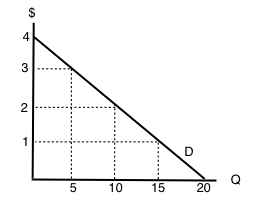
3. If the price of this good is $1 per unit, what will be the quantity demanded?
a) 5.
b) 10.
c) 15.
d) 20.
4. What are the TOTAL benefits to this individual if she consumes 10 units of the good?
a) $5.
b) $10.
c) $20.
d) $30.
5. The demand curve for a good is derived from the:
a) Marginal cost of the good.
b) Marginal benefit of the good.
c) Marginal benefits of the good minus marginal costs of the good.
d) Production Possibilities Frontier
6. Which of the following statements about demand curves is TRUE?
I. The “Law of Demand” holds if a consumer’s marginal benefit is lower at higher quantities consumed than it is at lower quantities consumed.
II. If the consumer’s marginal benefit is the same no matter what quantity is consumed, then her demand curve will be vertical.
III. All else equal, the marginal benefit of consuming a normal good will be higher for richer consumers than for poorer consumers.
a) III only.
b) I and II only.
c) I and III only.
d) I only.
The following FOUR questions refer to the diagram below, which illustrates a consumer’s demand curve for a good.
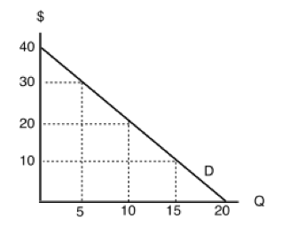
7. If the price of this good is $30, what quantity will be demanded?
a) 5 units.
b) 10 units.
c) 15 units.
d) 20 units.
8. If the price of this good is $20, what quantity will be demanded?
a) 5 units.
b) 10 units.
c) 15 units.
d) 20 units.
9. If the price of this good is $20, what will consumer surplus equal?
a) $100.
b) $200.
c) $300
d) $400.
10. If the price of this good falls from $30 to $20, but the consumer is prohibited from buying more than 5 units of the good, by how much will consumer surplus increase?
a) $100.
b) $75.
c) $50
d) $25.
