2.2 Production Possibility Frontier
Learning Objectives
By the end of this section, you will be able to:
- Understand how economic models work to simplify complex problems
- Define opportunity cost and apply it to daily situations
- Understand how to graph and analyze a PPF
- Explain how preferences influence our production decisions
Think of all the different variables that can impact trade. A country’s interest rate influences the flow of financial capital; its exchange rate encourages or discourages the purchase of goods and services. The weather can impact the production of goods, and politics can create tension between countries. Many of these examples are macro issues that will impact our micro analysis. How can we navigate such complex economic issues to make normative judgments? The answer is economic models.
An economic model is a simplified framework that is designed to illustrate complex processes. Oftentimes in introductory Microeconomics, these models seem oversimplified because they hold certain variables constant. While one should remain aware of this, these models are still useful. Holding some information constant can help us understand a concept without being overwhelmed by a vast number of influencing factors. Economic models are the building blocks of most modern economic theory. By understanding these models, we can develop a mindset to understand the economic world.
Model of Production

An economic model is only useful when we understand its underlying assumptions. For this model, imagine the following scenario:
You are stranded on a tropical island alone. On this island, there are only two foods: pineapples and crabs. In other words, you face a trade-off: any time you spend harvesting pineapples is time that cannot be spent looking for crabs. You are forced to make a decision on how to allocate the scarce resource of time.
While this is an extreme example, it is reflective of a common problem in production. Since there are only a certain number of hours in the day, time is a scarce resource. This scarcity limits the amount of total production.
Figure 2.2a displays a table showing several different combinations of goods that can be harvested in a given week. The table is very logical – if you spend all your time catching crabs, you will have no pineapples. Notice that you can produce either all crabs, all pineapples, or a mix of the two.
Assume you choose to only catch crabs. How many would have to be given up in order to obtain ten pineapples? In this example, only one. This is an important concept; even though our scarce resource is time, we can measure the cost of a good, in this case, pineapples, in terms of the foregone good, in this cases crabs.
This concept is called the Marginal Opportunity Cost of an action. In this case, since you have to give up one crab to produce 10 pineapples, the marginal opportunity cost for one pineapple is 1/10 of a crab.
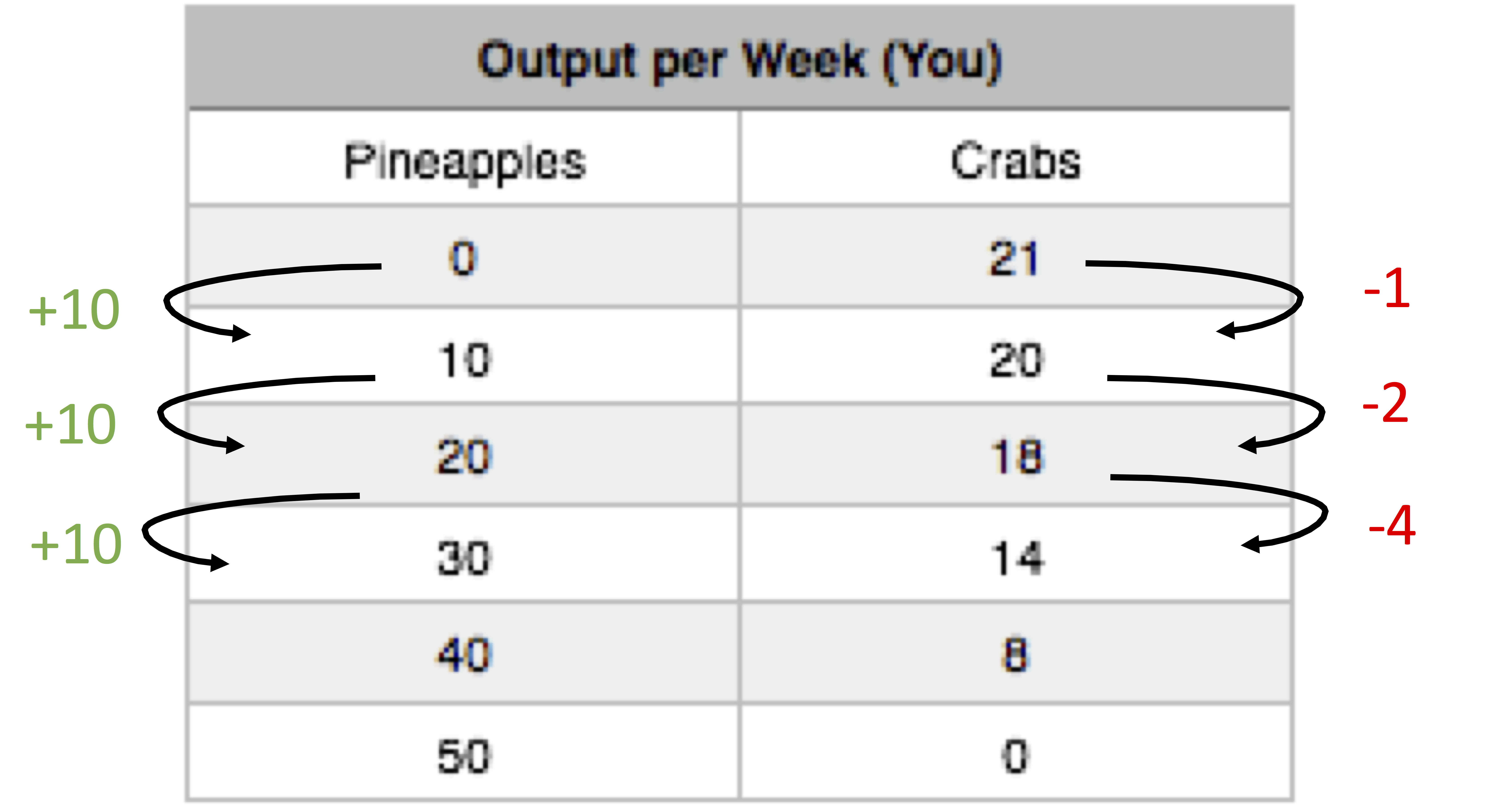
Notice how the marginal cost changes as you harvest more pineapples. To produce the next ten pineapples, it costs two crabs, and the next ten costs four. This continues until there are no more crabs to give up. While marginal opportunity cost is not always increasing, it is intuitive to think that the more pineapples you pick, the harder they will be to find, and therefore the more time you will have to give up to harvest 10 more.
Applications
 Opportunity Cost At University
The concept of “Opportunity Cost” is not just applicable when you are stranded on an island; in fact, we face opportunity costs every day. Consider the opportunity cost of reading this textbook. Perhaps for the hour you spend reading, you could have made $11 working at a restaurant, scrolled through Facebook, or spent time with friends. By continuing to read, you are forfeiting the opportunity of doing one of those things. One common fallacy when evaluating opportunity costs is considering all the different ways you could be spending your time. Remember, since you can only be in once place at a time, only the next best option is relevant in your decision making. In our simplified example, we limited our discussion to only two options so this fallacy did not interfere.
Production Possibility Frontier
While much useful analysis can be conducted with a chart, it is often useful to represent our models graphically. A Production Possibility Frontier (PPF) is the graphical representation of Figure 2.2a. It represents the maximum combination of goods that can be produced given available resources and technology. Each point represents one of the combinations from Figure 2.2a. In our example, while we would love to produce 50 pineapples and 50 crabs, this is out of our realm of possible production. In other words, it is not a point on our PPF.
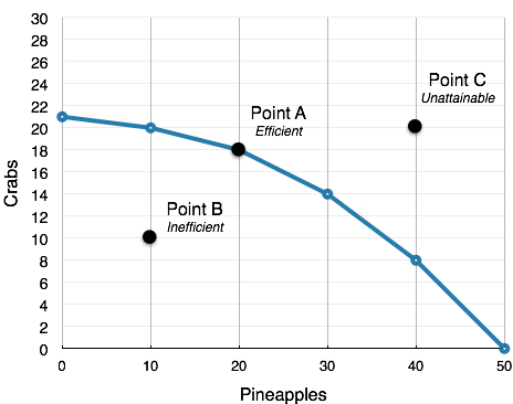
Using our terminology from before, each point along our PPF (i.e. Point A) is efficient (in a one-person world) since there is no way to get more pineapples without giving up some crabs and vice-versa. There are no Pareto Improvements in the current situation.
If we are inside the PPF (i.e. Point B), we are not fully using our resources. In this case, we can produce more pineapples without having to give up any more crabs. This point is inefficient.
Points outside the PPF (i.e. Point C), while preferable, are unattainable given constraints in resources and time.
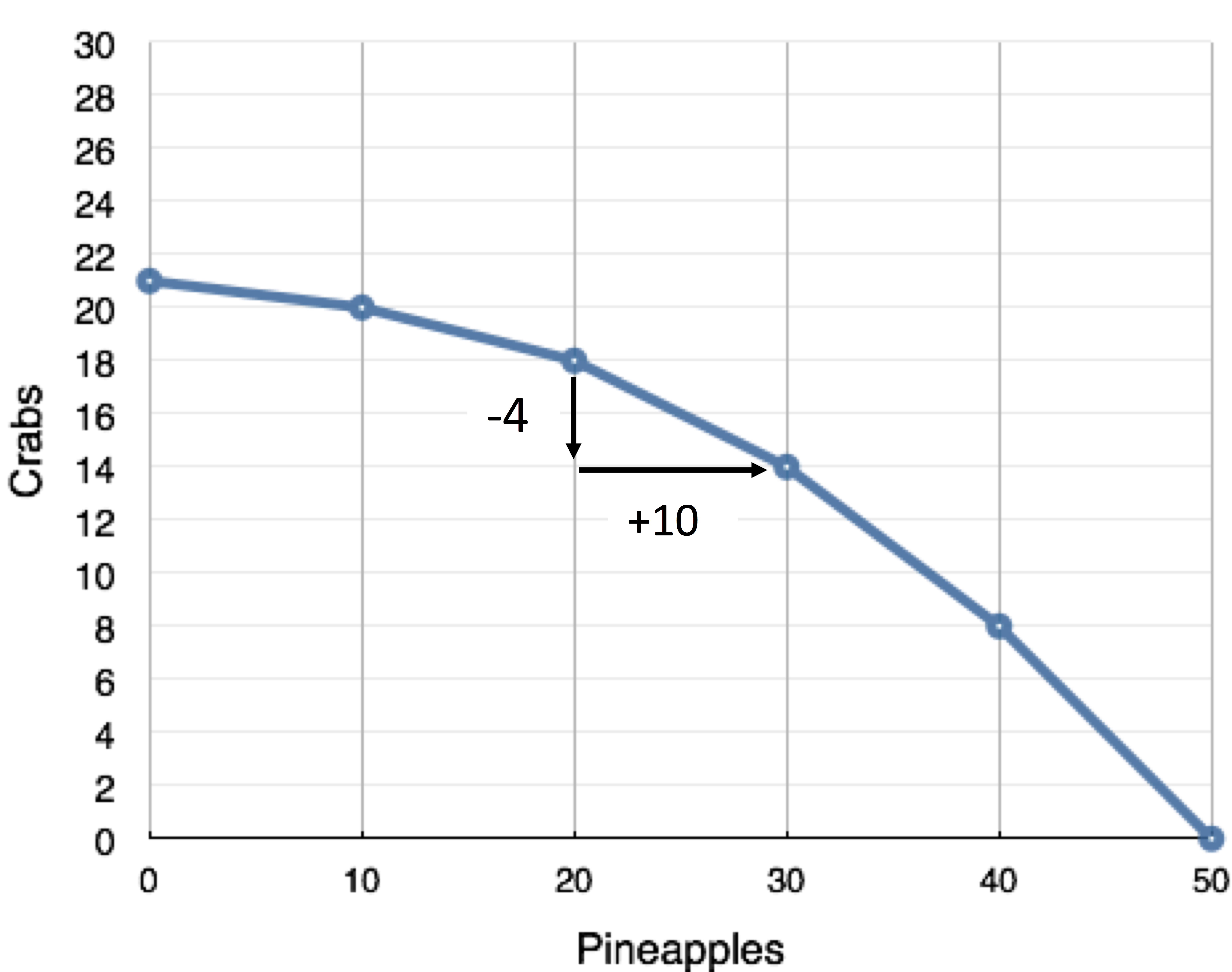
Using our analysis of Marginal Opportunity Cost (MC) from before, we see that the Slope (absolute value) of the PPF is the Marginal Cost of the good on the horizontal axis. Recall that slope is calculated using rise over run. By calculating the slope from (20,18) to (30,14), we see the MC is 4/10 of a crab for one pineapple (or 4 crabs for 10 pineapples as represented in our chart). As we move down the PPF, the slope and MC increase.
Given our scarce resources and time, we can efficiently produce any point along the PPF. Now, we face the same problem as before. How do we determine which bundle to choose? Is it better to produce 50 pineapples and 0 crabs, 21 crabs and 0 pineapples, or a mix of the two? This depends entirely on preferences. Perhaps you are allergic to crabs and they provide you no value, or maybe you have a desired ratio of crabs to pineapples. Since the bundles along the PPF are all efficient, we cannot pass judgment on which is best.
Applications
The Island Example – Brexit
While our discussion so far has referred to a deserted island scenario, the same concepts are easily relatable to a country’s production. On a much larger scale, countries face trade-offs in production. The island situation can be likened to a country with a policy of autarky – a state of economic independence or self-sufficiency. The United Kingdom’s decision to leave the European Union (commonly known as Brexit) metaphorically makes it more of an island. The country will have to face more trade-offs with the goods it can produce. As we will see in the next section, trade can reduce these trade-offs and allow countries to reach points outside their PPF.

Click to Learn More
Shifting a PPF
As we will see in Topic 2.3, trade allows countries, individuals, or firms to reach points outside their PPF. In addition to trade, there are some other factors that shift a countries PPF, allowing an change in attainable output. These factors include:
- A Shift in Technology – If you were to invent a computer system that showed the location of crabs and pineapples on the island, you would be able to produce more of both goods, shifting the PPF outward.
- More Education or Training – If you were to become more skilled at harvesting pineapples or crabs, your attainable output would increase, shifting the PPF outward.
- Natural Disaster – If disaster strikes, and pineapples or crabs become less plentiful, your attainable output would decrease, shifting the PPF inward.
These are not the only factors that could shift the PPF, but they are the most common. What is important to recognize is that a PPF represents what is attainable, and that is subject to change.
Glossary
- Autarky
- A state of economic independence or self-sufficiency.
- Economic Model
- A simplified framework that is designed to illustrate complex processes.
- Marginal Opportunity Cost
- A solution that is ethically or legally just and fair, but may not be wholly satisfactory to any or all the involved parties.
- Preferences
- The ordering of alternatives based on their relative utility, a process which results in an optimal choice.
- Production Possibilities Frontier (PPF)
- A diagram that shows the productively efficient combinations of two products that an economy can produce given the resources it has available.
Exercises 2.2
1. Consider the PPF diagram below.
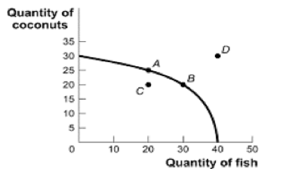
Given the PPF illustrated, what is the opportunity cost of moving from B to A?
a) 5 coconuts.
b) 10 fish.
c) 5/10 fish
d) 10/5 coconuts.
The following TWO questions refer the diagram below, which illustrates the PPF for a producer of two goods, x and y.
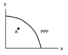
2. Which of the following statements is TRUE?
I. The marginal cost of producing x is higher at high levels of x than it is at low levels of x.
II. The marginal cost of producing y is higher at high levels of y than it is at low levels of y.
III. The marginal cost of producing both x and y is constant in the level of production.
a) I only.
b) II only.
c) III only.
d) I and II only.
3. If this economy is operating at point A, which of the following statements is TRUE?
I. The opportunity cost of producing more x is zero.
II. The opportunity cost of producing more y is zero.
III. Point A is inefficient.
a) III only.
b) I and II only.
c) I and III only.
d) I, II, and III.
The following TWO questions refer to the PPF diagram below.
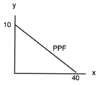
4. What is the MARGINAL cost of producing good y?
a) 1/4 of a unit of x.
b) 1/4 of a unit of y.
c) 4 units of x.
d) 4 units of y.
5. What is the cost of producing FOUR units of good y?
a) 16 units of x.
b) 4 units of x.
c) 1/4 of a unit of x.
d) 40 units of x.
6. Consider a PPF drawn with x on the horizontal axis and y on the vertical axis. Which of the following concepts can be used to explain why this production possibility frontier could be flat at relatively lows levels of x and steep at relatively high levels of x?
a) Increasing marginal costs.
b) Scarcity
c) Sunk costs.
d) Trade
7. Which of the following concepts can be used to explain why production possibility frontiers slope downwards.
a) Scarcity
b) Sunk costs.
c) Trade
d) Increasing marginal costs.
