5.2 Indirectly Correcting Externalities
Learning Objectives
By the end of this section, you will be able to:
- Explain how policy can improve societal outcomes when markets do not function perfectly.
- Compare and demonstrate how different environmental policies work to reduce pollution.
A Source of Market Failure
Recall from our analysis in Topic 5.1 that reducing the quantity in the market from the optimal market level of production to the socially optimal level of production raised social surplus. In Topic 4, we saw a variety of policies that changed the quantity from the market equilibrium and resulted in a deadweight loss. Why the difference?
In Topic 3 and 4, our supply and demand models relied on the assumption that the market was perfectly competitive and that there were no externalities. With these assumptions, the market would naturally optimize both the market and social surplus because there would be no external costs.
Recognizing that externalities do exist, our market no longer naturally optimizes, since external costs do not impact market participants and thus are not taken into account for their decision.
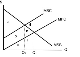
Recall this diagram of a negative externality. We found that social surplus at the optimal market quantity (or competitive equilibrium) was a-d. We then found that at the socially optimal level of production, the social surplus was a. We concluded that d was the deadweight loss from being at the competitive equilibrium and not addressing the externality. Since the market did not naturally maximize societal welfare, the unaddressed externality results in a market failure. Since our market equilibrium quantity differs from our social equilibrium quantity, we have a deadweight loss. When left unaddressed, externalities cause competitive markets to fail.
Correcting or ‘Internalizing’ an Externality
Now we know that an externality is a form of market failure that arises because market participants do not account for factors external to the market. This makes the market quantity is too low or too high relative to the socially optimal level of production. Fortunately, in Topic 3 and 4, we learned a variety of policies that influence the number of goods exchanged in a market. We can use these to set quantity where MSB =MSC. If we create policy correctly, we can bring the market back to the social surplus maximizing level of output.
We can either set the appropriate quantity directly through a quota, price floor, or price ceiling. More commonly, governments address the externality through a tax or subsidy. In this case, the government introduces a tax that will make market participants act as if they care about participants outside the market. In economic jargon, this is called internalizing the externality. A tax that addresses a negative externality by taxing the good instead of the actual external cost is called a Pigouvian Tax. We work through an example below.
Consider the following diagram of a perfectly competitive market with a negative externality present.
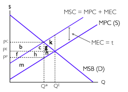
Zero Externality isn’t the Answer
Notice in the diagram above that at the socially optimal level of production, external costs do not equal zero. At QE, external costs are m+c+h+k+g+n. When we introduce a tax that takes us to Q*, external costs are equal to m+c+h. A common misconception is that introducing a tax in this market eliminates external costs. This is incorrect. In some sense, we are aiming for an “optimal” level of external cost. To get a sense for this, consider the manufacturing industry. We could get external costs (like the adverse effects of carbon dioxide emissions) to equal zero if we stopped production entirely, but then we would have a world with little energy.
Secondly, consider a world where the externality is not constant like in the previous example. Perhaps it is increasing in the level of production like the diagram below.
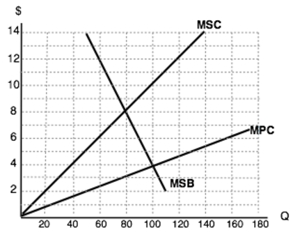
At this point, you should be able to convince yourself that the equilibrium quantity is 100 and the socially efficient level of output is 80. The intuition behind the policy response is the same as before, but we have to be careful about the amount of the tax as the marginal external cost is changing. We want to set the level of the tax equal to the marginal external cost at the socially efficient level of output. This value is 8-3 or $5. We know that setting a tax equal to $5 will bring us to 80 units, where social welfare is maximized.
Third, notice that we have been indirectly targeting pollution with the policies we have discussed. We have taxed the good to reduce pollution. There is no incentive to innovate our production processes and make them “greener” because no matter how green your good is, you will still have to pay the tax. In the next section, we look at policies that address this and directly target pollution.
Glossary
- Pigouvian Tax
- a tax levied on any market activity that generates negative externalities (costs not internalized in the market price)
Exercises 5.2
The following TWO questions refer to the diagram below, which illustrates the marginal private cost, marginal social cost, and marginal social benefits for a goods whose production results in a negative externality.
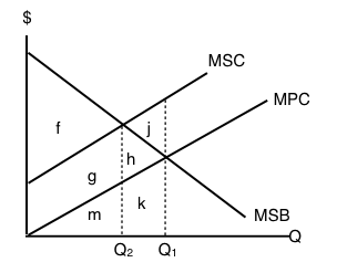
1. If the government introduces a per unit tax equal to the marginal external cost, what area represents the change in social surplus?
a) j; a decrease.
b) j; an increase.
c) h; a decrease.
d) h; an increase.
2. Which area represents external costs at the social-surplus-maximizing quantity of output?
a) External costs are zero.
b) g + h + j.
c) g + h.
d) g.
The following TWO questions refer to the diagram below, which illustrates the supply and demand curves for a perfectly competitive market. Assume that each unit of output results in a marginal external cost of $5.
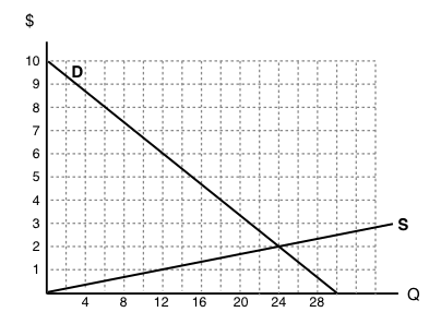
3. In the absence of government intervention, what will the deadweight loss equal?
a) $0.
b) $30.
c) $60.
d) There is insufficient information to determine the size of the deadweight loss.
4. If a tax of $5 per unit is introduced in the market illustrated above, then the price that consumers pay will be ____ and the price that producer receive (net of the tax) will be____.
a) $9; $4.
b) $8; $5.
c) $7; $6.
d) $6; $1.
