5.3 Directly Targeting Pollution
Learning Objectives
By the end of this section, you will be able to:
- Show how the government can directly target pollution.
- Consider the pros and cons of pollution standards, cap and trade, and pollution tax policies.
- Explain how firms respond to each policy.
In the previous section, we looked at externalities and policies to correct the market failures they cause. In this section, we look at mechanisms to directly target pollution.
Model Background:
Why do firms pollute? The economist’s answer is because there is a benefit to pollution – production implies pollution and production allows the firm to generate revenue. In an unregulated world, firms can maximize their profits by using the cheapest production method available. It is not an unreasonable assumption to say that the cheapest method is likely the “dirtiest” method. When producing, firms are weighing the MB of pollution (revenue) against the MC. In an unregulated world, the MC of pollution is zero, so firms will emit the maximum level of pollution that their production method allows for. The problem is that when a firm only looks at its own cost and benefits, the societal cost of pollution is ignored. Thus, we have a role for government intervention in addressing this market failure. In analyzing the decisions of firms directly around emission or pollution, we use the abatement model.
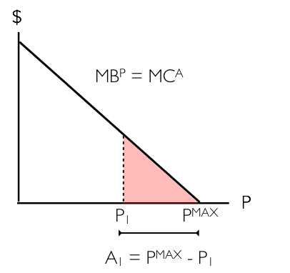
The graph above illustrates the marginal benefit of pollution (MPB), or equivalently, the marginal cost of abatement (MCA) for a firm. Abatement, a term describing the reduction of pollution, is almost always costly. On the vertical axis, we have cost and/or benefit in dollar terms. On the horizontal axis, we have pollution. Recall that in the absence of regulation, the firm will emit at PMAX. Assume this firm decides to reduce its emissions to P1. In this case, it would need to pay large amounts of money for abatement, since there would be a hefty cost associated with cleaning up its production. The area under the MCA curve between PMAX and P1, shown above as the red triangle, represents this cost.
It is important to note something about marginal cost of abatement. As shown in the diagram above, it is likely to be low at relatively high levels of P and high at relatively low levels of P. Consider a coal-fired power plant to understand why this is true. When the firm is making no efforts to reduce pollution, there are relatively cheap things it can do to reduce its pollution, like installing a smokestack scrubber. This concept is commonly referred to as “low-hanging fruit.” When this firm is polluting only a small amount, it is much costlier to reduce pollution by an additional unit. An extreme example is that the coal-fired power plant would need to convert to a wind farm.
In theory, we could map the marginal social cost of pollution onto the above graph, find the intersection and force the firm to reduce its emissions to this optimal level. However, there is a heavy information burden for this to happen. In order for this to occur, we would need to know social cost information and the cost of abatement for the firm. This is at best impractical and at worst impossible. In reality, we estimate the appropriate pollution reduction and create a policy to get us there.
There are three that we will consider: pollution standards, a pollution tax, and a cap-and-trade system.
In creating any policy, we want to consider three criteria:
First, we want to ensure low-cost opportunities for abatement are chosen over high-cost opportunities whenever possible. This will result in pollution reduction at the least cost.
Second, ideally, we want a system with a low informational burden. As we have discussed, assigning a cost to environmental impact is very difficult. If we can design a system that does not depend on these imprecise estimates, we can still get to a beneficial outcome.
Lastly, we want to think about distribution: Who is paying the cost for this policy and who is benefiting?
Pollution Standards
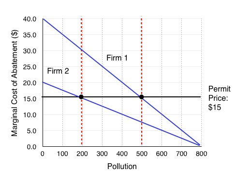
The most rudimentary policy available is called a pollution (or emission) standard. This policy directly limits the amount of pollution a firm is allowed to emit. In effect, the policymaker tells the firms that they all must restrict their emission to, for example, 350 units. The upside of this policy is that it ensures the government will reach its pollution reduction target. The bad news is that the reduction is unlikely to occur at least cost. Consider the Figure 5.3b, which shows two firms and their associated MCA below.
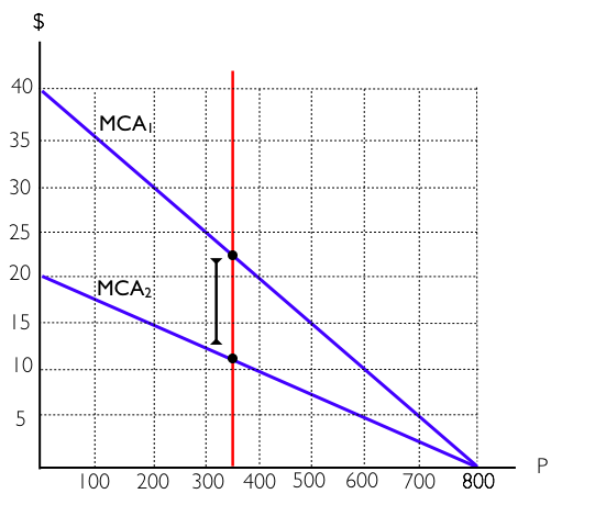
We can see that Firm 1 (with MCA1) has higher abatement costs over at all levels of P compared to Firm 2 (with MCA2).
Suppose the government wants to reduce pollution from PMAX = 1600 (800 from each firm) by 900 units. It decides to divide the abatement burden evenly between the two firms (450 each) so a pollution standard is set at 350 units. This means that each firm may only emit 350 units. This is shown on the diagram above.
From this policy, the government gets the desired reduction of emission by 900 units but not at least cost. Observe in the diagram that at a pollution level of 350 units, Firm 1 has a MCA of around $22 and Firm 2 has a MCA equal to around $11. This means that Firm 1 is willing to pay up to $22 for one more unit of pollution, and Firm 2 is willing to accept at least $11. If there was a way for Firm 1 to pay Firm 2 for some of its pollution allowance, then both parties could gain. This is not possible under the pollution standards regime.
Cap and Trade
A scheme where Firm 1 can buy pollution allowances from Firm 2 exists, and is called Cap and Trade. Under cap and trade, the government sets a certain pollution level and then provides permits that firms can purchase, sell, and trade. In effect, the government is creating a market for pollution and limiting the available pollution to the number of permits it provides. This allows the market to allocate emissions reduction efficiently.
Suppose the government wants the same 900-unit reduction in emissions and to reduce emissions to 700 units. Its first step is to create 700 permits. The second and more difficult decision is to decide how many permits each firm will get initially. Let’s assume each firm is given half the permits.
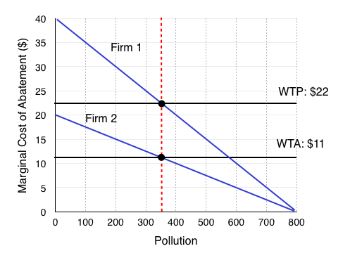
Figure 5.3c is the same diagram we had in our pollution standard scenario. As we noted, the MCA’s are not equal, and there is an incentive for Firm 1 to pay Firm 2 for some of its pollution allowance. Specifically, Firm 1 is willing to pay its MCA for an additional unit of pollution ($22), and Firm 2 is only willing to accept (WTA) more than its MCA ($11). Clearly, there are beneficial exchanges available.
What happens when a trade occurs? We can see that as pollution level changes, the MCA for each firm will change as well.
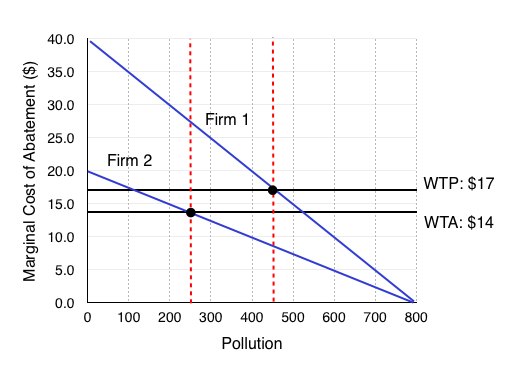
When Firm 1 increases its pollution by 100 units and Firm 2 decreases its pollution by 100 units, the parameters for a beneficial exchange have changed. Now, Firm 1 is only willing to pay up to $17 to pollute, and Firm 2 must be paid at least $14.
We can see that transactions will continue to occur until the WTP = WTA, or the MCA for each firm is the same. This occurs at $15.
What prices will permits trade at?

If there are a range of prices in which beneficial transactions can occur, for example in Figure 5.3c at any price between $11 and $22, what price will the permits trade at? Remember that in a perfectly competitive market, the price is set by the market. This means that the price of permits will equal the MCA at the equilibrium. Why? Our buying firms will be willing to pay somewhere between $22 and $15, and our selling firms need to be paid somewhere between $11 and $15. If you are a firm looking to sell your permit and you try to sell for more than $15, the buying firm will look elsewhere, knowing that other firms will sell for $15. If you are a buying firm and you offer less than $15, the selling firm will go elsewhere, knowing it can receive at least $15. Therefore, the equilibrium price of permits is $15.
The conclusion? We can easily find the permit price by finding the point where the marginal costs of abatement are the same, and the total amount of emissions is equal to the number of permits. By identifying this point, we will also be able to tell who is the buyer and seller of permits in each situation.
How Cap and Trade Minimizes Costs
We can look at how each firm assesses the benefits and costs of selling and buying permits and conclude that the exchange is mutually beneficially and results in a Pareto improvement. Having an open market for trading permits ensures that if one firm is more efficient at reducing emissions, it will sell permits to a firm that is less efficient. This ensures that pollution reduction is done in the most efficient way possible.
Consider Figure 5.3, which shows the benefits and costs of pollution for Firm 1 compared to the benefits and costs of abatement for Firm 2.
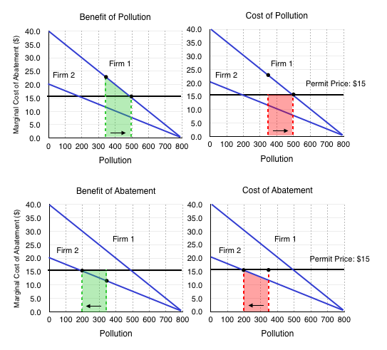
Clearly, issuing permits results in efficient emission reductions. In this policy, the government has to set a quantity, and allows the market to set the price of pollution.
Pollution Tax
There is one more method the government can use to directly curb pollution. Whereas with cap and trade, the government has to set the quantity of emissions, a pollution tax allows it to set the price.
Setting the price can be more difficult. If the government wants to reduce emissions to 700 units, it will have to set a tax rate that incentivizes firms to do so. With the diagrams above, this might not seem so difficult, but normally the government will not know the MCA of the firms.
All that considered, if the government has the information, a pollution tax can have much the same effect as cap and trade. If the government sets the pollution tax at $15, consider how Firm 1 behaves:
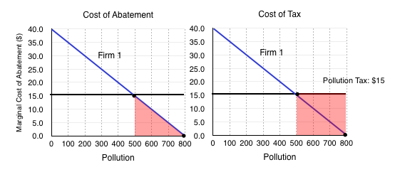
Without the tax, the firms both maximize their pollution. Once the $15 tax is set, the firms each compare the costs of abatement with the cost of paying the tax. In Figure 5.3d, we can see that it costs Firm 1 more to pay the tax than it does for them to reduce pollution from 800 units to 500 units.
This does not mean it will reduce pollution entirely. Consider Firm 1’s decision when it is emitting 500 units of pollution:
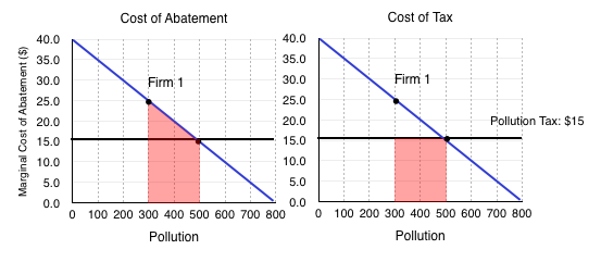
In this case, we see the cost of abatement is higher than the cost of the tax. This means that the firm will pay the tax. Notice that this causes Firm 1 to reduce emissions to the same level as under cap and trade. Doing the same analysis for Firm 2 would lead us to the same conclusion. This means that a pollution tax also causes firms to reduce emissions in the most efficient way possible.
Key Concepts and Summary
Examples of market-oriented environmental policies include taxes, cap and trade, and pollution reduction. These policies ensure those who impose negative externalities face the social cost. Consider the following table which summarizes the 3 policies:
| Is it Efficient? | Who Gains? | What decisions does government make? | |
| Pollution Standards | No | No one | The government has to set the rate of pollution.(quantity decision) |
| Cap and Trade | Yes | The more efficient firm can earn revenue. | The government has to decide how many permits to allocate.(quantity decision) |
| Pollution Tax | Yes | The government earns tax revenue. | The government has to decide on the tax rate.(price decision) |
Glossary
- Abatement
- reduction or lessening, in this case the reduction of pollution
- Cap and Trade
- a government program designed to cap the total level of emissions from firms by creating a market for pollution permits
- Pollution Allowance
- a permit that allows a firm to emit a certain amount of pollution; firms with more permits than pollution can sell the remaining permits to other firms
- Pollution Standard
- legal requirements that set limits on the permissible amount of pollutants, restrict the quantity of pollution that a firm emits
- Pollution Tax
- a tax imposed on the quantity of pollution that a firm emits
Exercises 5.3
Use the diagram below to answer the following THREE questions, which illustrates the marginal costs of abatement for two polluting firms.
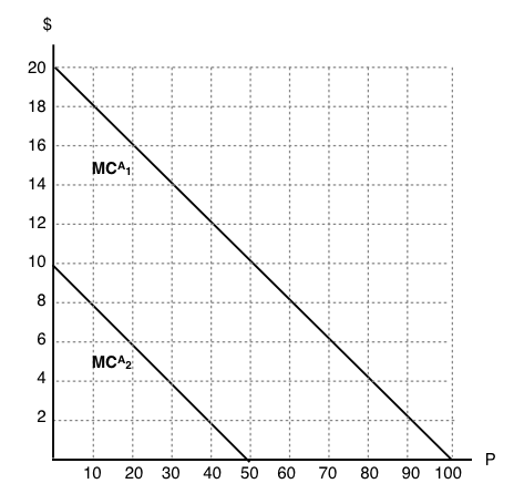
1. If the marginal private cost of pollution is zero for each firm then, in the absence of regulation, pollution levels will be:
a) P1 = 100, P2 = 100.
b) P1 = 50, P2 = 100.
c) P1 = 50, P2 = 50.
d) P1 = 100, P2 = 50.
2. If a pollution tax of $6 per unit is introduced, pollution levels will be:
a) P1 = 60, P2 = 10.
b) P1 = 70, P2 = 20.
c) P1 = 80, P2 = 30.
d) P1 = 90, P2 = 40.
3. Suppose a cap and trade program is introduced to reduce aggregate emissions. If each firm receives HALF the permits in the initial allocation, then which firm will sell permits and which firm will buy?
a) Firm 1 will sell permits and firm 2 will buy permits.
b) Firm 1 will buy permits and firm 2 will sell permits.
c) We need to know the number of permits in total, in order to figure out who will sell and who will buy.
d) We need to know the equilibrium price of permits, in order to figure out who will sell and who will buy.
The following THREE questions refer to the diagram below, which illustrates the marginal abatement cost curve for two firms. Assume these are the only two emitters of pollution.
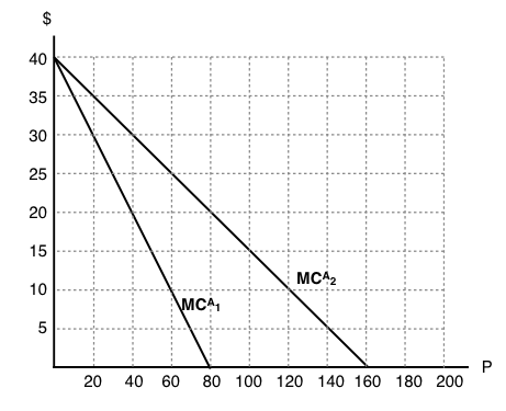
4. If a pollution tax of $10 per unit is introduced, then how much will each firm emit in the taxed equilibrium?
a) Firm 1 will emit 60 units, firm 2 will emit 120 units.
b) Firm 1 will emit 80 units, firm 2 will emit 160 units.
c) Firm 1 will emit 20 units, firm 2 will emit 40 units.
d) Each firm will emit no pollution.
5. If a cap and trade program is introduced in which aggregate emissions are restricted to 120 units, what is the competitive equilibrium price for permits?
a) $10.
b) $15.
c) $20.
d) We cannot determines the equilibrium price without knowing the initial distribution of permits.
6. Suppose a cap and trade program is introduced, in which firm 1 receives 100 permits and firm 2 receives 120 permits, in the initial allocation. Which of the following statements is true?
a) Given the initial allocation of permits, neither firm will want to buy permits.
b) Given the initial allocation of permits, neither firm will want to sell permits.
c) In equilibrium, firm 1 will buy permits and firm 2 will sell permits.
d) In equilibrium, firm 1 will sell permits and firm 2 will buy permits.
7. Which if the following statements about environmental policy is true?
I. A cap and trade policy allows the government to directly control the quantity of pollution, but the price of pollution is determined by private agents.
II. A carbon tax allows the government to directly control the price of pollution, but the quantity of pollution is determined by private agents.
III. Both carbon taxes and cap and trade programs will result in least-cost abatement.
a) I only.
b) II only.
c) I and II only.
d) I, II, and III.
The following two questions refer to the diagram below, which illustrates the marginal abatement cost curve for two polluting firms. Note that in the absence of regulation, each firm will emit 80 units of the pollutant in question, so that aggregate emissions are 160 units.
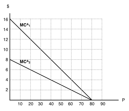
8. If a pollution tax of $8 per unit is introduced, then what is the percentage decrease in aggregate emissions?
a) 25%.
b) 50%.
c) 75%.
d) 100%.
9. If a cap and trade program is introduced in which aggregate emissions are restricted to 100 units, what be the equilibrium price of permits?
a) $2.
b) $4.
c) $6.
d) $8.
