6.2 The Indifference Curve
Learning Objectives
- Understand the indifference curve
- Explain the marginal rate of substitution
- Represent perfect substitutes, perfect complements, and convex preferences on an indifference curve
Understanding Preferences
Rational consumers will spend all of their income, meaning they will produce somewhere along their budget line. The point they produce ultimately depends on preferences. Consider again the situation of José, who can buy T-shirts or Movies.
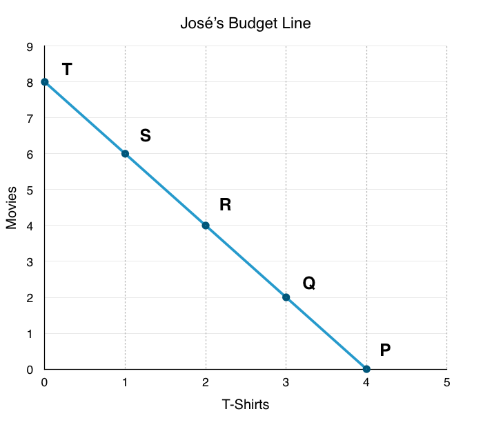
If José likes T-shirts but hates movies, he will spend all of his money on T-shirts and nothing on movies. In other words, he will select bundle P.
If José likes movies but hates T-shirts, he will spend all of his money on movies and none on T-shirts. In other words, he will select bundle T.
Usually, consumers prefer a mix of both goods. Where they consume depends on the strength of their preferences, measured by a concept known as utility. Utility, an economic term that was introduced by Daniel Bernoulli, refers to the total satisfaction received from consuming a good or service. Utility measures our happiness derived from consumption. Using the concept of utility, we can graph our preferences.
Graphing Preferences
In Topic 6.1, we looked at how to represent a consumer’s choices graphically with a budget line, with each point showing a different way for the consumer to spend all of their budget. Now, we want to represent their preferences on the same diagram.
An indifference curve maps the consumption bundles that the consumer views as equal. The consumer is equally as happy to consume at any point along the indifference curve.
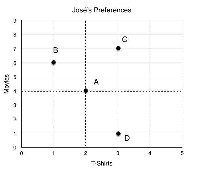
Consider Figure 3.2a, where several possible consumption points are laid out. With the knowledge we have, what can we say about José’s consumption choices? Assuming José is at point A, would he prefer another bundle more?
Point C – At point C José consumes more movies and T-shirts. Since more goods make José happier, he is better off at point C.
Point B – At point B, José consumes more movies, but fewer T-shirts. Because we do not know José’s preferences, we cannot say whether José is better or worse off.
Point D – At point D, José consumes more T-shirts, but fewer movies. Because we do not know José’s preferences, we cannot say whether José is better or worse off.
Perfect Substitutes
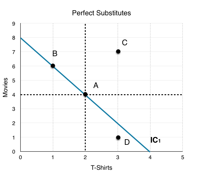
Let’s start with a simple example of José’s preferences and assume he views T-shirts and movies as nearly perfect substitutes. If the two goods were perfect substitutes, José would be indifferent between Movies and T-shirts. Let’s assume instead that José likes T-shirts twice as much as movies – José is equally as happy with 4 T-shirts as he is with 8 movies.
At point A, to keep utility constant, if José is to lose 1 T-shirt, he has to gain 2 movies to stay on the same indifference curve.
What information does this give us regarding José preferences between A, B, C and D?
Point C – Again, since José has more movies and T-shirts at point C, his utility has increased, and he is on a higher indifference curve.
Point B – At point B, José has one less T-shirt, but 2 more movies. As outlined, this means his utility is unchanged, and he is on the same indifference curve.
Point D – At point D, José has 1 more T-shirt, but 3 fewer movies. Since José only views T-shirts as two times more valuable than movies, his utility has decreased, and he is on a lower indifference curve.
It is important to recognize that there is an infinite amount of indifference curves. We can graph an IC for point D, and an IC for point C.
Since very point on an indifference curve represents equal utility, we can be confident that every point on IC2 is superior to every point on IC1, and every point on IC1 is superior to every point on IC0.
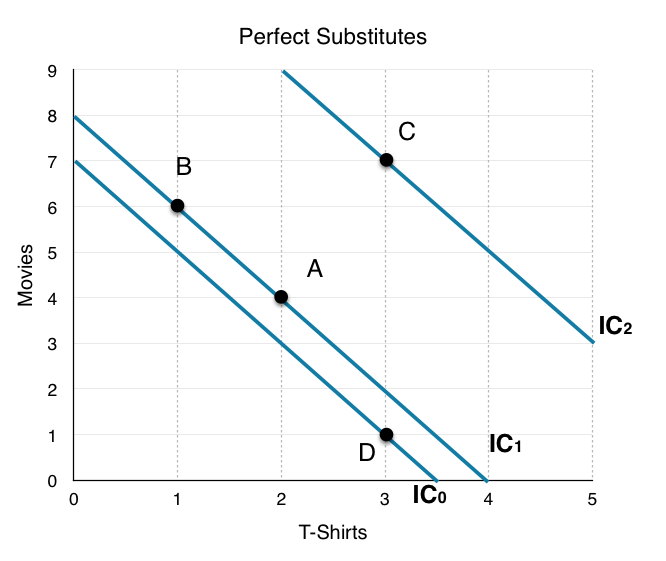
To maximize his utility, José will choose to consume on the highest possible indifference curve that he can afford.
What Does Slope Mean?
The slope of the indifference curve is the marginal rate of substitution (MRS). The MRS is the amount of a good that a consumer is willing to give up for a unit of another good, without any change in utility. In the example above, our MRS is equal to -2. This means that the maximum amount of movies José is willing to give up to get one T-shirt is 2. If he were to give up any more, he would be on a lower indifference curve. Likewise, if he were to give up any less, he would be on a higher indifference curve.
Since indifference curves are downward sloping, they have a negative slope. Because we know the definition of MRS, keeping the negative sign is unnecessary. We can just use the absolute value of the slope to simplify the analysis.
Convex Preferences
Thinking about José’s preferences, it may seem odd to simply state that he values T-shirts twice as much as movies. What if José has no T-shirts and 8 movies? In this case, perhaps he would be willing to give up more movies to obtain a T-shirt. This intuition that consumers prefer variety leads us to an indifference curve that is strictly convex. At low levels of x, we prefer it more than at high levels of x and vice versa for good y.
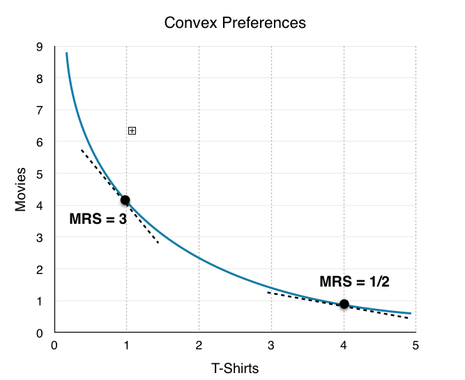
Figure 6.2d shows an example of José’s convex preferences. Notice how the MRS changes depending on the consumption. When José has few T-shirts, he is willing to give up more movies in exchange for one more shirt. Conversely, when José has many T-shirts, he is not willing to give up as many movies to obtain one more T-shirt.
Graphically, when José has 1 T-shirt and 4 movies, he is willing to give up to 3 movies in exchange for 1 T-Shirt. (MRS = 3)
When José has 4 T-Shirts and 1 Movie he is only willing to give up 1/2 a movie in exchange for 1 T-Shirt. (MRS = 1/2)
In this example, José has diminishing MRS. In other words, the more of one good he consumes, the smaller the MRS becomes for that good.
Conclusion
We said earlier that José wants to be on the highest indifference curve possible, given his budget. By putting our budget line and indifference curve on the same diagram and maximizing José’s utility given his constraints, we can find exactly where he will consume.
Glossary
- Diminishing Marginal Rate of Substitution
- The more of a good one consumes, the less desirable it becomes. Represented by MRS falling as x increases on an indifference curve.
- Indifference Curve
- a graph representing all consumption opportunities that a consumer holds as equal value
- Marginal Rate of Substitution
- the rate at which a consumer is willing to give up one good for another without a change in utility; the slope of the indifference curve
- Strictly Convex Preferences
- a good becomes less desirable as you acquire more of it, preference for a variety of goods
- Utility
- economic term referring to the total satisfaction received from consuming a good or service
Exercises 6.2
1. If a consumer (who buys two goods) has strictly convex preferences, then:
a) Her indifference curves are relatively steep at low levels of x and relatively flat at high levels of x.
b) Her preference is to have some of each of the two goods, rather than all of one and none of the other.
c) Her marginal rate of substitution diminishes.
d) All of the above are true.
2. The diagram below illustrates the indifference curve of a consumer of goods x and y.
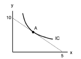
Assuming the current consumption bundle is the point labelled A, which of the following statements is TRUE?
a) This consumer is just willing to give up 2 units of y for an additional x.
b) This consumer is just willing to give up 1 unit of y for an additional 2 units of x.
c) This consumer is just willing to give up 1/2 a unit of x for an additional y.
d) Both a) and c) are true.
3. A consumer has $20 per week to spend on coffee and muffins. The price of a cup of coffee and the price of a muffin both equal $1 each. If the consumer always likes to consume one muffin for every cup of coffee he drinks, what consumption bundle will maximize his utility?
a) 20 muffins and no coffee.
b) 20 coffees and no muffins.
c) 10 coffees and 10 muffins.
d) All of the above consumption bundles maximize his utility – he is indifferent among all those options listed.
