4.1 Calculating Elasticity
Learning Objectives
By the end of this section, you will be able to:
- Calculate the price elasticity of demand
- Calculate the price elasticity of supply
- Calculate the income elasticity of demand and the cross-price elasticity of demand
- Apply concepts of price elasticity to real-world situations

That Will Be How Much?
Imagine going to your favorite coffee shop and having the waiter inform you the pricing has changed. Instead of $3 for a cup of coffee with cream and sweetener, you will now be charged $2 for a black coffee, $1 for creamer, and $1 for your choice of sweetener. If you want to pay your usual $3 for a cup of coffee, you must choose between creamer and sweetener. If you want both, you now face an extra charge of $1. Sound absurd? Well, that is the situation Netflix customers found themselves in 2011 – a 60% price hike to retain the same service.
In early 2011, Netflix consumers paid about $10 a month for a package consisting of streaming video and DVD rentals. In July 2011, the company announced a packaging change. Customers wishing to retain both streaming video and DVD rental would be charged $15.98 per month – a price increase of about 60%. In 2014, Netflix also raised its streaming video subscription price from $7.99 to $8.99 per month for new U.S. customers. The company also changed its policy of 4K streaming content from $9.00 to $12.00 per month that year.
How did customers of the 18-year-old firm react? Did they abandon Netflix? How much will this price change affect the demand for Netflix’s products? The answers to those questions will be explored in this chapter with a concept economists call elasticity.

Anyone who has studied economics knows the law of demand: a higher price will lead to a lower quantity demanded. What you may not know is how much lower the quantity demanded will be. Similarly, the law of supply shows that a higher price will lead to a higher quantity supplied. The question is: How much higher? This topic will explain how to answer these questions and why they are critically important in the real world.
To find answers to these questions, we need to understand the concept of elasticity. Elasticity is an economics concept that measures the responsiveness of one variable to changes in another variable. Suppose you drop two items from a second-floor balcony. The first item is a tennis ball, and the second item is a brick. Which will bounce higher? Obviously, the tennis ball. We would say that the tennis ball has greater elasticity.
But how is this degree of responsiveness seen in our models? Both the demand and supply curve show the relationship between price and quantity, and elasticity can improve our understanding of this relationship.
The own price elasticity of demand is the percentage change in the quantity demanded of a good or service divided by the percentage change in the price. This shows the responsiveness of the quantity demanded to a change in price.
The own price elasticity of supply is the percentage change in quantity supplied divided by the percentage change in price. This shows the responsiveness of quantity supplied to a change in price.
Our formula for elasticity, [latex]\frac{\%\Delta Quantity}{\%\Delta Price}[/latex], can be used for most elasticity problems, we just use different prices and quantities for different situations.
Why percentages are counter-intuitive
Recall that the simplified formula for percentage change is [latex]\frac{New\;Value-Old\;Value}{Old\;Value}[/latex], also written as [latex]\frac{\Delta Value}{Old\;Value}[/latex].
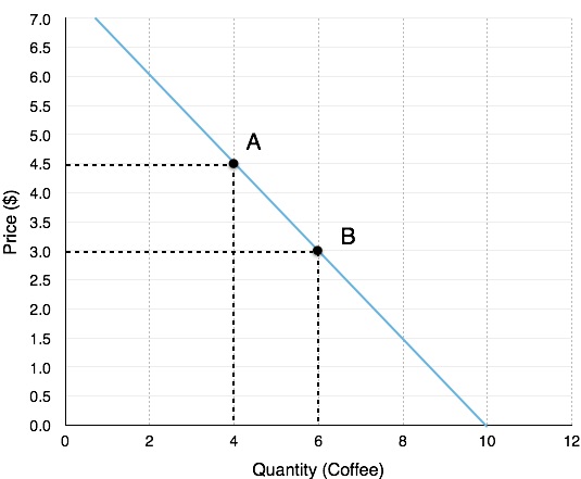
Suppose there is an increase in quantity demanded from 4 coffees to 6 coffees. Calculating percentage change ([latex]\frac{\left(6-4\right)}{4}[/latex]) there has been a 50% increase in quantity demanded. Using the same numbers, consider what happens when quantity demanded decreases from 6 coffees to 4 coffees, ([latex]\frac{\left(4-6\right)}{6}[/latex]) this change results in a 33% decrease in quantity demanded.
Right away, this should raise a red flag about calculating the elasticity between at two points, if percentage change is dependant on the direction (A to B or B to A) then how can we ensure a consistent elasticity value?
Let’s calculate elasticity from both perspectives:
Moving from A to B:
%ΔPrice: The coffee price falls from $4.50 to $3.00, meaning the percentage change is [latex]\frac{\left(3.00-4.50\right)}{4.50}[/latex] = -33%. Price has fallen by 33%.
%ΔQuantity: The quantity of coffee sold increases from 4 to 6, meaning the percentage change is [latex]\frac{\left(6-4\right)}{4}[/latex] = 50%. Quantity has risen by 50%
Elasticity: [latex]\frac{\%\Delta Quantity}{\%\Delta Price}=-\frac{50\%}{33\%}[/latex] = 1.5*
Moving from B to A:
%ΔPrice: The coffee price rises from $3.00 to $4.50, meaning the percentage change is [latex]\frac{\left(4.50-3.00\right)}{3.00}[/latex] = 50%. Price has risen by 50%.
%ΔQuantity:
The quantity of coffee sold falls from 6 to 4, meaning the percentage change is [latex]\frac{\left(4-6\right)}{6}[/latex] = -33%. Quantity has fallen by 33%
Elasticity: [latex]\frac{\%\Delta Quantity}{\%\Delta Price}=\frac{33\%}{50\%}[/latex] = 0.67
These two calculations give us different numbers. This type of analysis would make elasticity subject to direction which adds unnecessary complication. To avoid this, we will instead rely on averages.
*Note that elasticity is an absolute value, meaning it is not affected by positive of negative values.
Mid-point Method
To calculate elasticity, instead of using simple percentage changes in quantity and price, economists use the average percent change. This is called the mid-point method for elasticity, and is represented in the following equations:
The advantage of the mid-point method is that one obtains the same elasticity between two price points whether there is a price increase or decrease. This is because the denominator is an average rather than the old value.
Using the mid-point method to calculate the elasticity between Point A and Point B:
[latex]\begin{array}{r @{{}={}} l}\%\;change\;in\;quantity & \frac { { 6 }-{ 4 } }{ ({ 6 }+{ 4 })/2 } \times 100 \\[1em] & \frac { 2 }{ 5 } \times 100 \\[1em] & 40\% \\[1em] \%\;change\;in\;price & \frac { { 3.00 }-{ 4.50 } }{ ({ 3.00 }+{ 4.50 })/2 } \times 100 \\[1em] & \frac { -1.50 }{ 3.75 } \times 100 \\[1em] & -40\% \\[1em] Price\;Elasticity\;of\;Demand & \frac { 40\% }{ 40\% } \\[1em] & 1 \end{array}[/latex]
This method gives us a sort of average elasticity of demand over two points on our curve. Notice that our elasticity of 1 falls in-between the elasticities of 0.67 and 1.52 that we calculated in the previous example.
Point-Slope Formula
In Figure 4.1a we were given two points and looked at elasticity as movements along a curve. As we will see in Topic 4.3, it is often useful to view elasticity at a single point. To calculate this, we have to derive a new equation.
[latex]\frac{\%\Delta Quantity}{\%\Delta Price}=Elasticity[/latex]
Since we know that a percentage change in price can be rewritten as
[latex]\frac{\Delta Price}{Price}[/latex]
and a percentage change in quantity to
[latex]\frac{\Delta Quantity}{Quantity}[/latex]
we can rearrange the original equation as
[latex]\frac{\frac{\Delta Quantity}{Quantity}}{\frac{\Delta Price}{Price}}[/latex]
which is the same as saying
[latex]\frac{\Delta Quantity\cdot Price}{\Delta Price\cdot Quantity}=\frac{\Delta Q}{\Delta P}\cdot \frac{P}{Q}[/latex]
This gives us our point-slope formula. How do we use it to calculate the elasticity at Point A? The P/Q portion of our equation corresponds to the values at the point, which are $4.5 and 4. The ΔQ/ ΔP corresponds to the inverse slope of the curve. Recall slope is calculated as rise/run.
In Figure 4.1, the slope is [latex]\frac{3-4.5}{6-4}[/latex] = 0.75, which means the inverse is 1/0.75 = 1.33. Plugging this information into our equation, we get:
[latex]\frac{\Delta Q}{\Delta P}\cdot \frac{P}{Q}[/latex]
[latex]1.33\cdot \frac{4.5}{4}[/latex] = 1.5
This analysis gives us elasticity as a single point. Notice that this gives us the same number as calculating elasticity from Point A to B. This is not a coincidence. When we are calculating from Point A to Point B, we are actually just calculating the elasticity at Point A, since we are using the values on Point A as the denominator for our percentage change. Likewise from Point B to Point A, we are calculating the elasticity at Point B. When we use the mid-point method, we are just taking an average of the two points. This solidifies the fact that there is a different elasticity at every point on our line, a concept that will be important when we discuss revenue.
Not Really So Different
Even though mid-point and Point-Slope appear to be fairly different formulas, mid-point can be rewritten to show how similar the two really are.
[latex]\frac{\frac{\Delta Q}{(Q1+Q2)/2}}{\frac{\Delta P}{(P1+P2)/2}}[/latex] = [latex]\frac{\frac{\Delta Q}{Q1+Q2}}{\frac{\Delta P}{P1+P2}}[/latex]
Remember that when a fraction is divided by a fraction, you can rearrange it to a fraction multiplied by the inverse of the denominator fraction.
= [latex]\frac{\Delta Q}{\Delta P}\cdot \frac{\left(P1+P2\right)}{\left(Q1+Q2\right)}[/latex]
Notice that compared to point-slope: [latex]\frac{\Delta Q}{\Delta P}\cdot \frac{P}{Q}[/latex], the only difference is that point-slope is the inverse of the slope multiplied by a single point, whereas mid-point is the inverse of the slope multiplied by multiple points. This reinforces the conclusion that mid-point represents an average.
Other Elasticities
Remember, elasticity is the responsiveness of one variable to changes in another variable. This means it can be applied to more that just the price-quantity relationship of our market model. In Topic 3 we discussed how goods can be inferior/normal or substitutes/complements. We will examine this even further when we introduce consumer theory, but for now we can develop our understanding by applying what we know about elasticities.
Own-price elasticity of supply (ePS)
Our analysis of elasticity has been centred around demand, but the same principles apply to the supply curve. Whereas elasticity of demand measures responsiveness of quantity demanded to a price change, own-price elasticity of supply measures the responsiveness of quantity supplied. The more elastic a firm, the more it can increase production when prices are rising, and decrease its production when prices are falling. Our equation is as follows:
[latex]\frac{\%\Delta Q\;Supplied}{\%\Delta P}[/latex]
Own-price elasticity of supply can be calculated using mid-point and point-slope formula in the same way as for ePD.
Cross-price elasticity of demand (eXPD)
Whereas the own-price elasticity of demand measures the responsiveness of quantity to a goods own price, cross-price elasticity of demand shows us how quantity demand responds to changes in the price of related goods. Whereas before we could ignore positives and negatives with elasticities, with cross-price, this matters. Our equation is as follows:
[latex]\frac{\%\Delta Q\;Good A}{\%\Delta P\;Good B}[/latex]
Consider our discussion of complements and substitutes in Topic 3.3. We defined complements as goods that individuals prefer to consume with another good, and substitutes as goods individuals prefer to consume instead of another good. If the price of a complement rises our demand will fall, if the price of a substitute rises our demand will rise. For cross-price elasticity this means:
A complement will have a negative cross-price elasticity, since if the % change in price is positive, the % change in quantity will be negative and vice-versa.
A substitute will have a positive cross-price elasticity, since if the % change in price is positive, the % change in quantity will be positive and vice-versa.
This adds another dimension to our discussion of complements/substitutes. Now we can comment on the strength of the relationship between two goods. For example, a cross-price elasticity of -4 suggests an individual strongly prefers to consume two goods together, compared to a cross-price elasticity of -0.5. This could represent the cross-price elasticity of a consumer for a hot dog, with respect to ketchup and relish. The consumer might strongly prefer to consume hot dogs with ketchup, and loosely prefers relish.
Income elasticity of demand (eND)
In Topic 3 we also explained how goods can be normal or inferior depending on how a consumer responds to a change in income. This responsiveness can also be measured with elasticity by the income elasticity of demand. Our equation is as follows:
[latex]\frac{\%\Delta Q}{\%\Delta Income}[/latex]
As with cross-price elasticity, whether our elasticity is positive or negative provides valuable information about how the consumer views the good:
A normal good will have a positive income elasticity, since if the % change in income is positive, the % change in quantity will be positive and vice-versa.
A inferior good will have a negative income elasticity, since if the % change in income is positive, the % change in quantity will be negative and vice-versa.
The value of our elasticity will indicate how responsive a good is to a change in income. A good with an income elasticity of 0.05, while technically a normal good (since demand increases after an increase in income) is not nearly as responsive as one with an income elasticity of demand of 5.
Summary
Elasticity is a measure of responsiveness, calculated by the percentage change in one variable divided by the percentage change in another.
Both mid-point and point-slope formulas are important for calculating elasticity in different situations. Mid-point gives an average of elasticities between two points, whereas point-slope gives the elasticity at a certain point. These can be calculated with the following formulas:
| Base Formula | Mid-Point Formula | Point-Slope Formula |
| [latex]\frac{\%\Delta Quantity}{\%\Delta Price}[/latex] | [latex]\frac{\Delta Q}{\Delta P}\cdot \frac{\left(P1+P2\right)}{\left(Q1+Q2\right)}[/latex] | [latex]\frac{\Delta Q}{\Delta P}\cdot \frac{P}{Q}[/latex] |
Since elasticity measures responsiveness, it can also be used to measure the own-price elasticity of supply, the cross-price elasticity of demand, and the income elasticity of demand. These can be calculated with the following formulas:
| Own-Price Elasticity of Supply | Cross-Price Elasticity of Demand | Income Elasticity of Demand |
| [latex]\frac{\%\Delta Q\;Supplied}{\%\Delta P}[/latex] | [latex]\frac{\%\Delta Q\;Good A}{\%\Delta P\;Good B}[/latex] | [latex]\frac{\%\Delta Q}{\%\Delta Income}[/latex] |
Glossary
- Cross-price elasticity of demand
- the percentage change in the quantity demanded of good A as a result of a percentage change in price of good B
- Elasticity
- an economics concept that measures responsiveness of one variable to changes in another variable
- Income elasticity of demand
- the percentage change in quantity demanded of a good or service as a result of a percentage change in income
- Own-price elasticity of demand
- percentage change in the quantity demanded of a good or service divided the percentage change in price
- Mid-point Method
- Involves multiplying the inverse of the slope by the values of a single point.
- Own-price elasticity of supply
- percentage change in the quantity supplied divided by the percentage change in price
- Point Slope Method
- A method of calculating elasticity between two points. Involves calculating the percentage change of price and quantity with respect to an average of the two points.
Exercises 4.1
1. Use the demand curve diagram below to answer the following question.
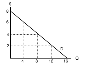
What is the own-price elasticity of demand as price increases from $2 per unit to $4 per unit? Use the mid-point formula in your calculation.
a) 1/3.
b) 6/10.
c) 2/3.
d) None of the above.
2. Suppose that a 2% increase in price results in a 6% decrease in quantity demanded. Own-price elasticity of demand is equal to:
a) 1/3.
b) 6.
c) 2
d) 3.
3. If own-price elasticity of demand equals 0.3 in absolute value, then what percentage change in price will result in a 6% decrease in quantity demanded?
a) 3%
b) 6%
c) 20%.
d) 50%.
4. Suppose you are told that the own-price elasticity of supply equal 0.5. Which of the following is the correct interpretation of this number?
a) A 1% increase in price will result in a 50% increase in quantity supplied.
b) A 1% increase in price will result in a 5% increase in quantity supplied.
c) A 1% increase in price will result in a 2% increase in quantity supplied.
d) A 1% increase in price will result in a 0.5% increase in quantity supplied.
5. Suppose that a 10 increase in price results in a 50 percent decrease in quantity demanded. What does (the absolute value of) own price elasticity of demand equal?
a) 0.5.
b) 0.2.
c) 5.
d) 10.
6. If goods X and Y are SUBSTITUTES, then which of the following could be the value of the cross price elasticity of demand for good Y?
a) -1.
b) -2.
c) Neither a) nor b).
d) Both a) and b).
7. If pizza is a normal good, then which of the following could be the value of income elasticity of demand?
a) 0.2.
b) 0.8.
c) 1.4
d) All of the above.
8. If goods X and Y are COMPLEMENTS, the which of the following could be the value of cross price elasticity of demand?
a) 0.
b) 1.
c) -1.
d) All of the above could be the value of cross price elasticity of demand.
