7.2 Understanding Producer Theory
Learning Objectives
By the end of this section, you will be able to:
- Calculate fixed costs, producer theory, and profits.
- Identify when firms will exit in the short-run.
- Be able to identify break-even and shut-down points.
Now that we have built our model for Producer Theory, we want to use it as a tool to understand how individual firms behave when faced with different prices. First, let’s see the different variables we can calculate from our graph.
Fixed Cost
In Topic 7.1, we showed that ATC = AVC + AFC. This means that AFC = ATC – AVC. Since FC = (AFC x Q), on our graph, we can find what total fixed costs are by simply multiplying the difference in AVC and ATC by the quantity at that level [(ATC-AVC) x (Q)].
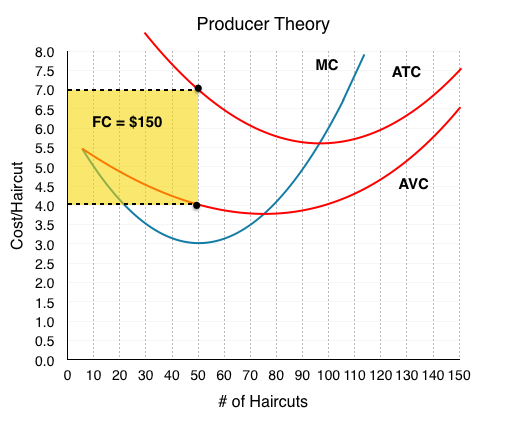
At Q = 50, our ATC = $7 and AVC = $4. Calculating fixed cost, we see it equals $150 [(7-4) x (50)], as stated in Topic 7.1. Remember that we derived ATC using fixed costs. Now, without knowing fixed cost, we can work backwards from our diagram to calculate total fixed cost at any Q.
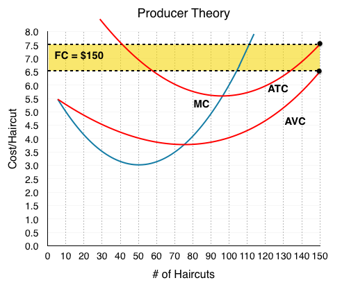
Calculating FC at any other point, we will find that it is always equal to $150. At Q = 150, ATC = $7.5 and AVC = $6.5. [(7.5-6.5) x (150)] = $150. Remember that fixed cost is always equal to $150 regardless of quantity, but AFC is always decreasing, as this $150 gets spread out across more goods.
The Competitive Firm
While we will use producer theory for non-competitive markets, for now, we are looking at price-taking firms.
If The Clip Joint is operating in a city with many other identical barber shops, they will lose their ability to set prices. A market price will dictate where they produce. We already know how this takes place. In Topic 1, we learned that economic agents use marginal analysis to make decisions about whether to increase a behaviour. If MB > MC, they will increase Q, and stop when MB = MC.
In this case, our price is our marginal benefit, since the price the firm receives is equal to the marginal revenue from an action. If price is $7, then every Q will earn the firm $7 of revenue. This means that P = MR = MB. Knowing that a firm maximizes producer surplus when MC = MB, we can now see that for a competitive firm, this occurs when P = MC.
When There’s Profits
Marginal analysis certainly maximizes producer surplus, but what about profits? Recall that producer surplus does not subtract fixed cost. This means that:
PS = TR – VC = (P – AVC) × Q.
Π = (P – ATC) × Q.
The only difference between PS and profit is fixed cost. Even though profits and producer surplus are not the same, the act of maximizing PS maximizes profits as well. Our marginal analysis tells us to increase production if ∆PS >∆VC (MB>MC). Since fixed costs do not change, the ∆PS = ∆Π and the analysis of ∆ Π >∆VC will be identical.
Let’s bring this understanding to our graph. Consider a market where The Clip Joint faces a price of $7.5. Using marginal analysis, we will produce until MC = P, or where our price line intersects our marginal cost. This occurs at Q = 110.
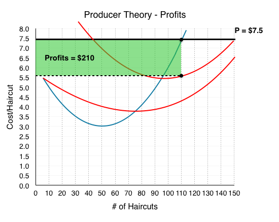
Calculating profits, with Π = (P – ATC) × Q, we find Π = (7.5 – 5.59) x 110 = $210.
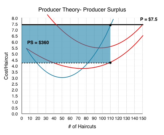
Calculating producer surplus, with PS = (P – AVC) × Q, we find Π = (7.5 – 4.23) x 110 = $360.
Note that our AVC and ATC are always calculated from the quantity where MC = P, as this is the profit maximizing quantity.
What is the difference between profits and producer surplus? Calculating $360 – $210, we find our fixed cost value of $150. This is no surprise – producer surplus is just our earnings before we subtract the fixed costs!
When There’s Losses
In the last example, The Clip Joint made healthy profits of $210 per day because P > ATC. In the long run, this will not be sustainable. In fact, firms will produce in the short-run even when P < ATC and Π is negative. Consider how The Clip Joint will behave when P = $5.
At P = $5, MC = MB when Q = 90. This means ATC = $5.5 and AVC = $3.83.
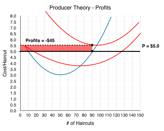
Calculating profits, with Π = (P – ATC) × Q, we find Π = (5.0 – 5.5) x 90 = -$45.
Why doesn’t the firm just shut down if it is losing money? Because it could be losing more money. Remember that no matter how much The Clip Joint produces, it still has to pay $150 in fixed costs. In this case, The Clip Joint will take a loss of $45 over a loss of $150.
We can come to the same conclusion by looking at producer surplus.
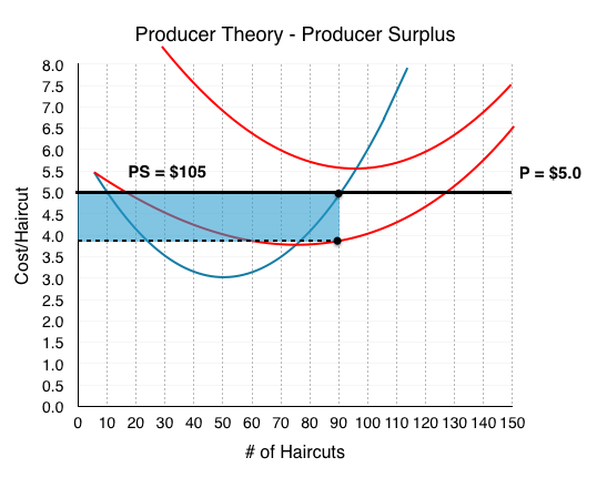
If PS > 0, then the firm has enough money to pay for all of its variable costs, plus some money left over to pay for its fixed costs. In this case, after paying VC, The Clip Joint has $105 left over to pay off a portion of its fixed costs.
This should clear up the relationship between FC, PS, and Profits. Producer Surplus is the amount we have before paying our fixed costs.
Smart-thinking company presidents do not continue to accept loses in the long run – that would be bad business. When the lease comes up for renewal, The Clip Joint will shut down knowing that it loses $45 from each day of business. Is there any case where it would shut down immediately in the short run? Yes. In this example, our PS > 0 since P > AVC; this means that even though we are losing money, we are able to pay off some of our FC. What if P < AVC? In this case, our firm would not even be able to pay for its workers, let alone rent and other fixed costs. The more the firm produced, the more money it would lose. In this case, our firm will shut down immediately. For this reason, we call the point where P = AVCMIN the Shut-Down Point. If the price falls any lower, the firm will shut down immediately.
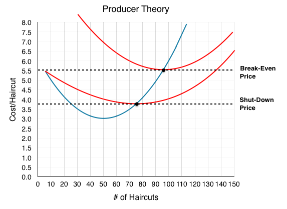
Another important point is the Break-Even Point where P = ATC. If the price falls below this, we reach a situation like the example above, where the firm makes negative profits but continues to operate in the short-run.
We have now analyzed how an individual firm behaves in the short-run in depth – but what about the long run? What happens when shocks to the economy cause price to change? We will answer these questions in Topic 7.3.
Glossary
- Break-Even Point
- A point where a firm is making no profits
- Shut-Down Point
- A point where a firm is only able to cover their variable costs of production
Exercises 7.2
1. Suppose you are given the following information about a competitive firm:
At the current quantity produced, P = $10; AVC = $4; AVC is at is minimum.
Given this:
a) The firm should continue to produce its current level of output; this is profit maximizing.
b) In order to maximize profits, the firm should increase output.
c) In order to maximize profits, the firm should decrease output.
d) We do not have enough information to determine what the firm should do to maximize profits.
2. If a firm’s profit equals $600 and its producer surplus equals $1,000, then its fixed costs:
a) Equal $400
b) Equal $600.
c) Equal $1,600.
d) Cannot be determined without further information.
The following TWO questions refer to the diagram below. Assume perfect competition.
3. The firm’s shut-down price is ____.
a) $2.
b) $4.
c) $7.
d) $10.
4. (Remember to refer to the diagram on the previous page.) The firm’s break-even price is ____.
a) $2.
b) $4.
c) $7.
d) $10.
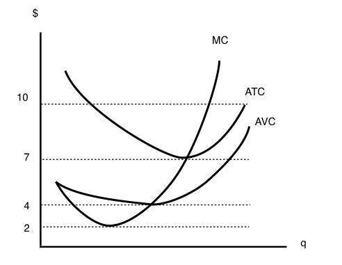
The following THREE questions refer to the diagram below, which illustrates a competitive firm’s cost curves.
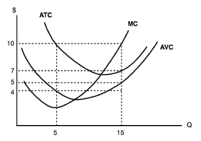
5. What do this firm’s fixed costs equal?
a) There is insufficient information to calculate the firm’s fixed costs.
b) $50.
c) $30.
d) $20.
6. (Remember to refer to the diagram on the previous page.) If this firm can sell its output for $10 per unit, then its maximum profit is equal to:
a) $150.
b) $75.
c) $60.
d) $45.
7. (Remember to refer to the diagram on the previous page.) If this firm can sell its output for $10 per unit, then its maximum producer surplus is equal to:
a) $150.
b) $75.
c) $60.
d) $45.
The following THREE questions refer to the diagram below. Assume perfect competition.
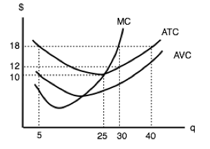
8. Given a price of $18, the profit-maximizing level of output for this firm is:
a) 5.
b) 25.
c) 30.
d) 40.
9. (Remember to refer to the diagram on the previous page.) Given a price of $18, the firm’s maximum profit is equal to:
a) $360.
b) $240.
c) $180.
d) $0.
10. (Remember to refer to the diagram on the previous page.) What do this firm’s fixed costs equal?
a) $0
b) $40.
c) $180.
d) There is insufficient information to calculate fixed costs.
