3.5 Other Determinants of Supply
Learning Objectives
By the end of this section, you will be able to:
- Understand the difference between supply and quantity supplied
- Know the four main determinants of supply
- Explain supply shifts from both horizontal and vertical perspectives
- Know the difference between explicit and opportunity costs

It’s as Easy as Cake
In section 3.4 we looked at the impact of price on the supply curve, but there are many other factors that affect a company’s decision to produce. For example, new innovations are always coming out to make cake decorating and baking easier, whether it is machines like the one shown above, or faster and better mixers. These inventions save time and energy at different levels of production. External forces like these impact our supply curve. The four supply shocks we will examine in detail include:
- Input Prices
- Technology
- Expectations
- Number of Producers
Whereas changes in price change quantity supplied, these factors shift supply. This is distinctly different from changes in quantity supplied as these shocks affect the price-quantity interaction at every point on our curve.
Is supply the same as quantity supplied?
As with demand and quantity demanded, supply is not the same as quantity supplied. When economists talk about supply, they mean the relationship between a range of prices and the distinct quantities supplied, as illustrated by a supply curve. When economists talk about quantity supplied, they mean only a certain point on the supply curve. Like demand, this means a change in quantity supplied is very different than a change in supply.
A change in supply refers to a shift in the supply curve, affecting the whole diagram and every interaction between price and quantity
A change in quantity supplied refers to a movement along the supply curve, exploring different points on the same curve.
We examined changes in quantity supplied in Topic 3.4. In this section, we discuss changes in supply.
Input Prices
Perhaps the most obvious shock to the supply curve is the cost of inputs. Also known as ‘Factors of Production’, these are the combination of labor, materials, and machinery used to produce goods and services. Our cupcake supply curve was based on the assumption of specific implicit and explicit costs which are prone to change. Any changes to these costs will affect our marginal costs at every point.
Changes in Explicit Costs
Changes in explicit costs are the easiest to conceptualize. We determined that the explicit cost of our cupcake supplies was around $0.50 each. What if icing sugar, an input to cupcakes, becomes more expensive? This will raise our marginal costs at all points of production, causing an upward shift in our supply curve.
Changes in Opportunity Costs
Opportunity cost is more of an abstract concept to think about in terms of input prices. Essentially, if cookies become more profitable to produce, our supply model considers the higher opportunity cost as an increase in our cost of making cupcakes. Suppose the market price for cookies increases from the original $0.50 to $1.00. Now, our MC will be as follows:
MC of 1st 5 cupcakes = $0.5 (explicit) + $0.8 (implicit) = $1.3 (increased from $0.9)
MC of 2nd 5 cupcakes = $0.5 (explicit) + $1.6 (implicit) = $2.1 (increased from $1.3)
MC of 3rd 5 cupcakes = $0.5 (explicit) + $2.4 (implicit) = $2.9 (increased from $1.7)
Notice this increase in marginal cost occurs at all levels, meaning the change will shift the entire supply, changing the quantity supplied at every point.
How does the supply curve actually change? In our discussion of demand, we explained that you could view a demand shift as vertical, as consumers’ willingness to pay changes at every quantity demanded; or as horizontal, as the amount consumers buy changes at every price level. There is a similar process for supply.
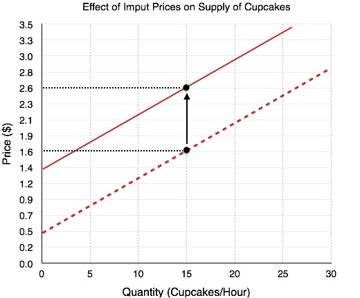
Vertical Shift – Figure 3.5a
The first way to view a shift in supply is as a vertical shift. Recall that supply represents the producer’s MC at each point of production. Assuming that in the original supply curve our MC of producing 15 units is $1.60, if costs increase by a dollar, we will see the marginal cost increase to $2.60. Since input prices increase by a dollar regardless of our production level, the entire curve will shift up by $1.00.
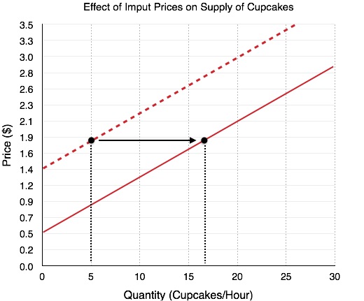
Horizontal Shift – Figure 3.5b
The next way to view a supply shift is slightly less intuitive. In Figure 3.5b, when the price of cupcakes is $1.80, our quantity supplied is equal to five cupcakes. Consider how this will change with a $1.00 decrease in input prices. Originally, we produced 5 cupcakes because our price was equal to marginal costs at that level When our costs fall, our price is still $1.80, but our costs are $0.90. Since P>MC, it is efficient to produce more than 5 units. Using marginal analysis, we find it is efficient to produce 17 units at this price.
Whereas before, it was only viable to produce 5 units at the price of $1.80, we can now produce up to 17 units efficiently. This causes the supply curve to shift right.
Most shocks will cause a uniform shift as can be explained vertically or horizontally. Technology, expectations, and the number of producers will all shift the supply curve in the same way as depicted.
Technology
As mentioned at the beginning of the section, changes in technology will also shift the supply curve. Why is that the case? Technology changes have a direct impact on the cost of production. If suddenly a new innovation allows you to cut your work time in half, you will cut down your costs of labor. If technology allows you to conserve wasted resources, then your input prices will decrease, These changes will increase supply, shifting the curve to the right. Technological Decay is a less common case where technological progress is reversed. What if the city banned the use of a certain cupcake icing machine because the noise was bothering other residents? This would cause you to go back to the less efficient practice of icing by hand, thereby increasing your costs. In summary:
- Improvements in technology will lower costs of production and increase supply
- Decay in technology will increase costs of production and decrease supply
Expectations
Like demand, expectations of the supply price affect production decisions. Production decisions are a lot like playing the stock market; if we are producing cupcakes and cookies to sell to the store tomorrow, we have to produce based on the current, incomplete knowledge we have about those prices. Normally, you will be confident that these prices will stay relatively stable, but if you have reason to believe the prices of cupcakes will drastically rise in the morning, you may devote more of your attention to producing them. Expectations are usually based on some form of evidence or signal and can cause supply shifts quite suddenly. In summary:
- If the firm expects prices to rise, supply will increase
- If the firm expects prices to fall, supply will decrease
Number of Producers
The final determinant of supply is the number of producers. So far, we have examined just one firm. Recall in section 3.3 we showed that the competitive market is characterized by many potential buyers, and added up individual demand curves to produce aggregate demand. Likewise, the market is made up of many other producers. By adding all the suppliers together, we get aggregate supply. This can affect total supply. If for example, four new firms enter the cupcake market, whereas Alaythia Cakes was producing just 5 cupcakes, now the firms each produce 5 cupcakes for a total of 25 (assuming that the individual supply curves are the same, which need not be the case). In summary:
- When more firms enter the market, supply will increase
- When firms leave the market, supply will decrease
Summary
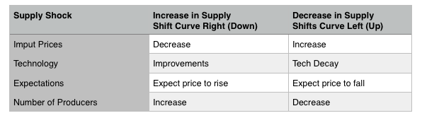
The four supply shocks have been summarized in the table below. Once again, the best way to learn these shifts is not to memorize them, but to practice shifts on the diagram to view their effects.
Glossary
- Aggregate Supply
- total of all goods and services (including exports and imports) supplied at every price level, within a national economy during a given period. Also called total output
- Explicit Costs
- direct costs of production such as rent, salaries, wages, or other input costs. Easily recognizable for classification and recording
- Factors of Production
- the combination of labor, materials, and machinery that is used to produce goods and services; also called inputs
- Implicit Costs
- the opportunity costs of an action, associated with an actions trade-offs
- Shift in Supply
- when a change in some economic factor (other than price) causes a different quantity to be supplied at every price
Exercises 3.5
1. Which of the following will NOT shift the market supply curve of good X?
a) A change in the cost of inputs used to produce good X.
b) A change in the technology used to produce X.
c) A change number of sellers of good X.
d) A change in the price of good X.
2. Which of the following is NOT a determinant of the supply of good X?
a) The cost of inputs used to produce good X.
b) The technology used to produce X.
c) The number of sellers of good X.
d) All of the above are determinants of the supply of good X.
The following TWO questions refer to the diagram below.
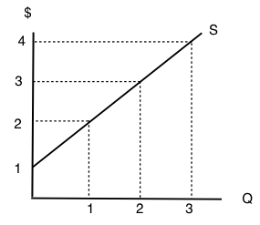
3. At what price will quantity supplied equal 3 units?
a) $1.
b) $2.
c) $3.
d) $4.
4. At what price will producer surplus equal $2?
a) $1.
b) $2.
c) $3.
d) $4.
5. A decrease in supply is, graphically, represented by:
a) A leftward shift in the supply curve.
b) A rightward shift in the supply curve.
c) A movement up and to the right along a supply curve.
d) A movement down and to the left along a supply curve.
6. Which of the following is NOT a determinant of the supply of good X?
a) The cost of labor used to produce good X.
b) The price of good X.
c) The income of consumers who buy good X.
d) The number of sellers of good X.
7. Which of the following is NOT a determinant of the supply of good X?
a) The cost of labor used to produce good X.
b) Consumer preferences.
c) Technology.
d) All of the above are determinants of the supply of good X.
8. Martin is selling his viola. The minimum amount he needs to be paid for the viola is $15,500. He find a buyer for who is willing to pay $22,400, but this buyer insists that Martin pays for delivery of the viola. The cost of delivery is $700. Martin’s producer surplus from selling his viola is equal to _____.
a) $14,800.
b) $7,600.
c) $6,900.
d) $6,200.
9. Which of the following statements about inferior goods is/are FALSE?
I. Inferior goods are those that we will never buy, no matter how cheap they are.
II. Inferior goods are those that we buy more of, if we become poorer.
III. Inferior goods are those that we buy more of, if we become richer.
a) I only
b) III only.
c) I and III only.
d) I, II, and III.
