8.1 Monopoly
Learning Objectives
- Understand the Marginal Revenue curve and its significance for a monopolist
- Describe how a monopoly chooses price and quantity
- Calculate the profits of a monopolist and explain why profits do not cause entry
- Explain why monopolies cause deadweight loss
Whereas perfect competition is a market where firms have no market power and they simply respond to the market price, a monopolistic market is one with no competition at all, and firms have complete market power. In the case of monopoly, one firm produces all of the output in a market. Since a monopoly faces no significant competition, it can charge any price it wishes. While a monopoly, by definition, refers to a single firm, in practice, the term is often used to describe a market in which one firm has a very high market share.
Even though there are very few true monopolies in existence, we deal with some every day, often without realizing it: your electric and garbage collection companies for example. Some new drugs are produced by only one pharmaceutical firm—and no close substitutes for that drug may exist.
While a monopoly must be concerned about whether consumers will purchase its products or spend their money on something altogether different, the monopolist need not worry about the actions of other firms. As a result, a monopoly is not a price taker like a perfectly competitive firm. Rather, it exercises power to choose its market price.
Competitive Market Recap
Below is Figure 7.3a to remind us how the competitive firm operates.
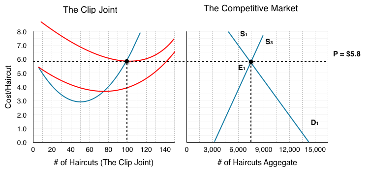
Notice in the competitive market, demand is downward sloping, but how does demand behave for the individual firm?
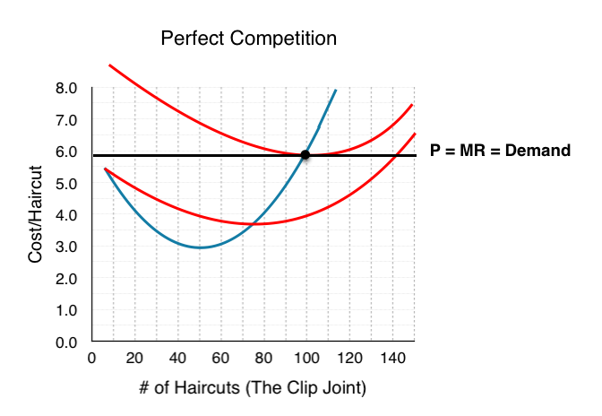
In Figure 8.1a the competitive market for an individual firm is re-created. Since the firm cannot deviate from the market price dictated by aggregate supply and demand, they face an elastic demand curve. If they raise the price, they will sell no units; if they drop the price, they will sell an infinite amount of units. Why don’t they drop price and sell more units? Remember that the firm produces where P = MR = MC, so if they sell beyond this point, they are losing money. This brings the market to equilibrium at the break-even point, where ATC is minimized and profit = 0.
Single Price Monopoly
So we know a competitive market faces an elastic demand, what about a single-priced monopoly? This is distinct from other monopolies in that the firm must charge the same price to all consumers. In this case, the aggregate demand is the firm’s demand! To explore monopoly, consider the sunglasses market.
What do Oakley, Ray-Ban and Persol have in common? They are all owned by the same brand. That’s right, Luxottica, an Italian based eyewear company, produces about 70% of all name brand eyewear. This is fairly close to a monopoly, as with that high of a market share, Luxottica dominates the market price. Notice that Luxottica is not a single price monopoly, as it practices a form of price discrimination by having multiple brands aimed at different consumers. Let’s consider what would happen if Luxottica only sold one kind of sunglasses at the same price to all consumers, and if they owned 100% of the market.
Whereas the competitive firm was a small player in the aggregate market, the monopolist dictates both the final price and the quantity. If Luxottica decides to lower price, it must do so for ALL buyers. Consider what implications this has on revenue.
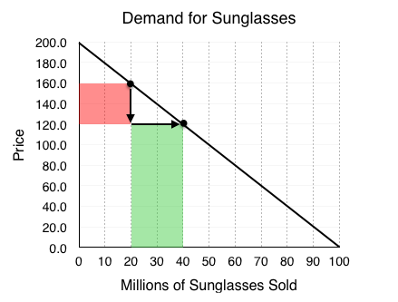
In Figure 8.1b the global demand for sunglasses is shown. According to the law of demand, as price falls, quantity demanded increases. This means that Luxottica can increase revenue by lowering price, as they sell more sunglasses. This is not that happens from a price decrease however, as the firm decreases price it loses some of the revenue on the goods it was previously selling.
At point A, Luxottica is selling 20 million sunglasses at $160 per pair. When it reduces the price to $120, two things happen:
- Luxottica loses $40 on each of the 20 million sunglasses it was selling before. 20 million consumers were willing to pay the full $160 for a pair, and now only have to pay $120. This results in a loss of $800 million for Luxottica. (shown as the red shaded region.
- Luxottica gains $120 on each of the 20 million new sunglasses it now sells. 20 million consumers were not willing to pay $160 for a pair, but are willing to pay $120. This results ina gain of $2.4 billion for Luxottica (shown as the green shaded region).
These changes collectively represent a net gain of $1.6 billion for Luxottica.
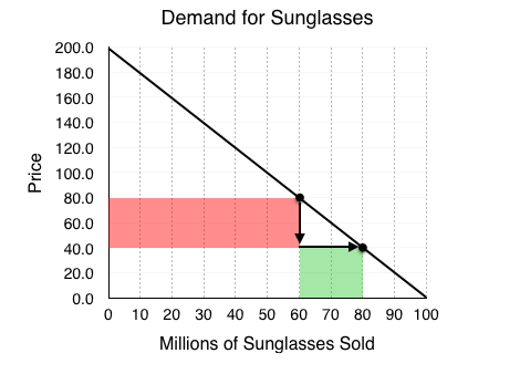
For a monopoly, a price decrease doesn’t always result in more revenue. When price is decreased, we have a loss in revenue from existing sales, and an increase in revenue from new sales. The more sales we are making, the greater the loss. Consider what happens when Luxottica drops prices when it is selling 60 million sunglasses.
At point A, Luxottica is selling 60 million sunglasses at $80 per pair. When it reduces the price to $40:
- Luxottica loses $40 on each of the 60 million sunglasses it was selling before. This results in a loss of $2.4 billion for Luxottica.
- Luxottica gains $40 on each of the 20 million new sunglasses it now sells. This results ina gain of $80 billion for Luxottica.
These changes collectively represent a net loss of $1.6 billion for Luxottica.
Representing Revenue
As we can see, finding where price = MC would no longer be a good metric for where we should produce, since we also want to take into account the affect price changes have on revenue. While the above analysis seems rather random, we can systematically represent the changes in revenue from a decrease in price – in fact, we already have! In Topic 4, we explored how the elasticity at different points along a demand curve affected the changes in revenue.
Remember, the equation to calculate elasticity is (% change in quantity/% change in price). Looking at the two changes in revenue from the examples above, we can see that the decrease in revenue came from the price change, and the increase came from the quantity change. This means that when % change in quantity > % change in price, our revenue increases from a price drop! Put simply, when our ED>1, we should continue to decrease price, maximizing our revenue. If ED<1, we have gone too far and can increase revenue by increasing price!
So, does this mean Luxottica will produce 50 million pairs of sunglasses, charge $100 per unit and call it a day? Not necessarily. While that would maximize revenue, remember that it doesn’t matter if revenue is rising if costs are rising by more. To find where we produce, we must find the point where marginal revenue = marginal cost.
Marginal Revenue
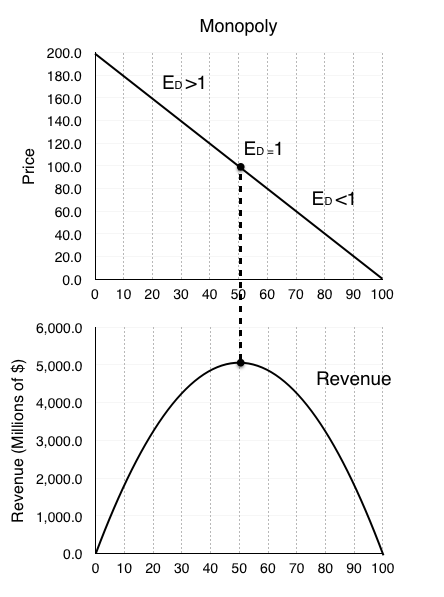
The amount that our revenue changes from an increase in quantity is called Marginal Revenue and can be represented alongside our demand curve. When ED >1, MR >0 since an increase in quantity will increase revenue. Conversely, When ED <1, MR <0 since an increase in quantity will decrease revenue.
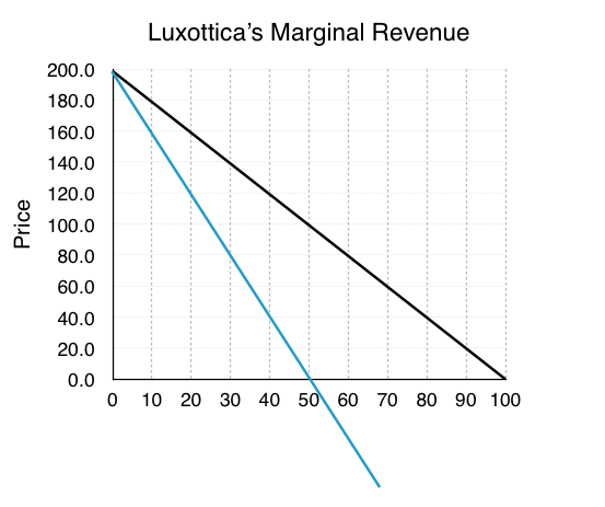
Since ED = 1 at the midpoint of a linear demand function, MR will always intercept the x-axis at QMAX/2, in this case at x=50. The key to this analysis is that whereas for the competitive firm P = MR, for a monopoly, P > MR.
Monopoly Behaviour
So what price will Luxottica charge? Adding its marginal cost to the graph, we can see that MC= MR at 30 million Sunglasses. At any quantity below this, MR > MC meaning Luxottica can increase profits by increasing production.
MR and MC intersect where P = $80, will this be the market price? At 30 million sunglasses sold, consumers are willing to pay $140 per pair. Luxottica knows this and will charge as high as it can. This means the market price will be $140.
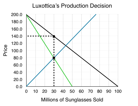
This behaviour is standard for a monopolist. Operate at the quantity where MC = MR, and charge a price equal to the consumers willingness to pay.
Market Surplus
In earlier topics, a key metric we analyzed was market/social surplus, which showed how government intervention can cause deadweight loss or correct the loss from externalities, etc. In this case, we want to see if a monopoly is as efficient as perfect competition. Recall our rule that differences in prices from equilibrium cause transfers and differences in quantity from equilibrium cause deadweight loss. Make a prediction as to how the monopoly market will affect efficiency.
Competitive Market
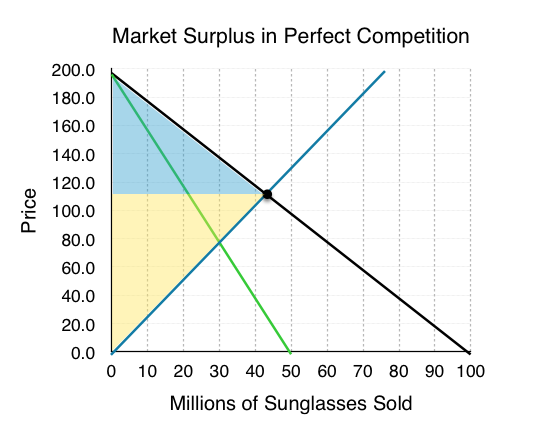
As a point of comparison, consider how this market would behave under perfect competition. Our equilibrium would be where MB (demand) = MC (supply). PE = $116, QE = 42 million.
Calculating market surplus:
Consumer Surplus = $1.764 billion
Blue shaded region.
[($200-$116)*(42)]/2 = 1.764 billion
Producer Surplus = $2.436 billion
Yellow shaded region.
[($116)*(42)]/2 = 2.436 billion
Market Surplus = $4.2 billion
Monopoly Market
In comparison, the monopoly market has PE = $140 and QE = 30 million.
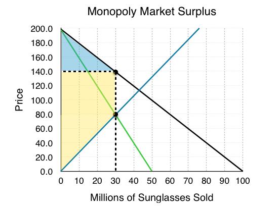
Calculating market surplus:
Consumer Surplus = $900 million
Blue shaded region.
[($200-$140)*(30)]/2 = 900 million
Notice consumer surplus decreased for two reasons. First, 12 million consumers are no longer willing to pay for the sunglasses (this quantity change will be part of the deadweight loss). Second, the 30 million consumers who still buy sunglasses now have to pay $60 more (the transfer from consumers to producers).
Producer Surplus = $3.0 billion
Yellow shaded region.
[($140-$80)*(30)] + [($80)*(30)]/2] = 3 billion
There are two changes to producer surplus with opposite effects. First, since 12 million consumers are no longer willing to buy the goods, Luxottica sells 12 million fewer sunglasses (this loss in surplus is the other piece of the deadweight loss). However, the $60 increase in price on the 30 million units it still sells more than compensates for the loss.
Market Surplus = $3.9 billion
Deadweight Loss from Monopoly
Remember that it is inefficient when there are potential Pareto improvements. In other words, if an action can be taken where the gains outweigh the losses, and by compensating the losers everyone could be made better off, then there is a deadweight loss. When we move from a monopoly market to a competitive one, market surplus increases by $1.2 billion. This means that the monopoly causes a $1.2 billion deadweight loss.
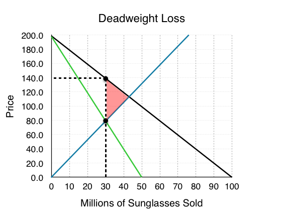
Remember that deadweight loss is only a result in deviations from the equilibrium quantity. Between 30 million sunglasses and 42 million sunglasses, consumers are willing to pay more than the firm’s marginal cost, so MB >MC. Since the monopolist is unwilling lower its price to increase output (and lose revenue from its pre-existing sales), the deadweight loss persists.
The red shaded region in Figure 8.1i is a measure of the loss to society from having monopoly rather than competition.
Glossary
- Marginal Revenue
- The increase in revenue resulting from a marginal increase in quantity
- Monopoly
- a situation in which one firm produces all of the output in a market
- Single-priced Monopoly
- a monopolist that can only charge one price
Exercises 8.1
1. Which of the following statements about a single-price monopoly is FALSE?
a) The monopolist will never charge a price on the inelastic portion of the demand curve.
b) Marginal revenue equals marginal cost at the profit-maximizing level of output.
c) Price equals marginal cost at the profit-maximizing level of output.
d) Marginal revenue is less than price, since the monopolist must lower its price to all consumers to sell an additional unit of output.
2. Suppose that at a monopolist’s current output choice, marginal cost equals price. Which of the following statements is TRUE?
a) The monopolist is currently maximizing profits.
b) The monopolist should produce more output to maximize profits.
c) The monopolist should produce less output to maximize profits.
d) We do not have enough information to know whether or not the monopolist is maximizing profits.
3. Refer to the diagram below, which illustrates the demand, marginal revenue, and marginal cost curves for a single-price monopolist.
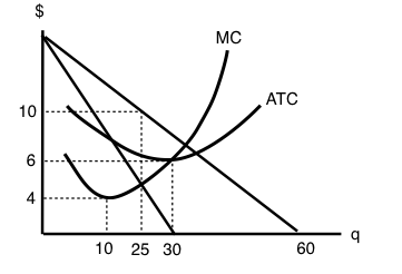
The profit-maximizing price and quantity for this monopolist are:
a) P = $4, Q = 60.
b) P = $6, Q = 60.
c) P = $4, Q = 30.
d) P = $10, Q = 25.
