Textbook or Burger?

In Topics 4.1 and 4.2, we looked at elasticity on a single demand curve and examined how responsive consumer are to price changes at various levels of production. But what about responsiveness across firms? Across industries? We know that in certain industries, such as the textbook industry, consumers are less responsive to change than others. How is the quantity demanded for textbooks affected by an increase in price? If the textbook for a course rose from $100 to $150, what would you do? Most students will buy the book anyway, since it is a required course material. Publishers are increasingly using different strategies to ensure the market stays inelastic or unresponsive to price change, such as bundling the textbook with mandatory course access codes. Compare this situation with the price of a burger. If the price of a burger rises from $8 to $12, you may purchase lunch from a different restaurant or start packing lunch from home. The market for textbooks and burgers are very different. In this section, we will explore the relative elasticity of different markets.

 Perfectly Elastic and Perfectly Inelastic

To begin the conversation about relative elasticity, it helps to first look at the extremes.

Perfectly Elastic

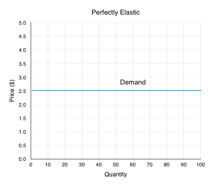
Imagine a product where if the price increased, even slightly, you wouldn’t buy any it anymore. Sound familiar? That’s because we introduced this concept in Topic 3, as one of the assumptions of a perfectly competitive market. One of the examples we used was identical hot dog stands, side by side, where the only difference was price. If quality is the same, the rational consumer will always purchase the hot dog that is a lower price. From the perspective of the stand, they know that if they increase price even slightly, they will sell 0 units. This means that E_D = ∞.

Using point-slope at any point in Figure 4.3a, we can confirm this.

[latex]\frac{\Delta Q}{\Delta P}\cdot \frac{P}{Q}=?[/latex]

We know that [latex]\frac{\Delta Q}{\Delta P}[/latex] is equal to the inverse of the slope. In the demand curve in Figure 4.3a, when the ΔP>0 then ΔQ is equal to ∞. This means that [latex]\frac{\Delta Q}{\Delta P}[/latex] = ∞. 

Perfectly Inelastic

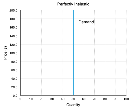
At the other end of the spectrum, consider a market where the firm can continue to increase prices with no change in quantity. If you were poisoned and had to buy the antidote, would you be responsive to price change? Probably not. This is an example of a situation where demand is nearly perfectly inelastic. If you increase the price, quantity demanded does not change. This means that E_D = 0.

We can confirm this by using point-slope at any point in Figure 4.4a.

In the demand curve in Figure 4.3a, when the ΔP>0 then ΔQ is equal to 0. This means that [latex]\frac{\Delta Q}{\Delta P}[/latex] = 0. 

 Relative Elasticity

The concepts of perfectly elastic and perfectly inelastic lead us into a discussion of relative elasticity. In 4.1 and 4.2, we examined a single demand curve, and looked at the numerical value of elasticity along that demand curve. However, elasticity can also be useful when comparing demand curves. Even though each demand curve has an inelastic, elastic, and unit elastic section, the comparison of the curves can show which markets are relatively more responsive to price changes. This is an important concept to understand for when we look at the impacts of a policy change.

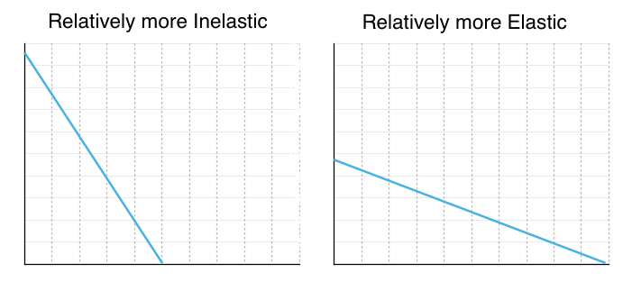
Figure 4.3c illustrates two curves. One is relatively more inelastic and the other is relatively more elastic. The best way to determine which is more elastic or inelastic is to compare each curve to the extremes. The curve more resemblant of perfect elasticity is relatively more elastic, the curve more resemblant or perfect inelasticity is relatively more inelastic.  Note this is different than saying one is elastic and the other inelastic! To emphasize this point, read the section “Bears and Elasticity.”

Bears and Elasticity

A bear jumps out of a bush and starts chasing two hikers. They both start running for their lives, but then one of them stops to put on his running shoes.

His friend says, “What are you doing? You can’t outrun a bear!”

His friend replies, “I don’t have to outrun the bear; I only have to outrun you!”

If both friends are trying to get away from the bear and you learn that one of them is fast, does this information tell you who gets eaten? No! It only matters which one is faster, or fast relative to the other. Relative elasticity is the same. In fact, we cannot pass judgement if one is elastic or inelastic unless we are referencing to another.

The concept of relative elasticity is not based on the calculations in 4.1 and 4.2, as each demand curve has an inelastic, elastic and unit elastic region. Demand curves take the shape of anything between perfectly elastic and perfectly inelastic, and you can only judge relative elasticity in reference to other curves.

What About Supply

The same concepts and principles can be applied to supply. There is fairly significant variation across different industries, with some relatively more elastic than others.

Factors That Influence Relative Elasticity

So what causes this difference in relative elasticity? For the most part, external factors which influence responsiveness.

Demand

1. Availability of substitutes

The availability of substitutes is a strong factor in determining the elasticity of a good. If there are many close substitutes, then it is fairly easy for consumers to find a suitable alternative to a good if prices rise.

2. Necessity of a good

In addition, the extent to which a good is a necessity or a luxury greatly influences its elasticity. Essentials, such as soap, flour, sugar, etc. are generally purchased in the same quantity regardless of price. On the other hand, consumers are very price conscious when it comes to luxury goods (such as comforts, jewelry, etc.).

3. Income

The necessity of a good depends quite heavily on the customer’s income. Someone with low income might be more price conscious (elastic) when purchasing a new sofa compared to someone with higher income. Generally the larger percentage of your income a good takes up, the more sensitive you will be to price changes.

Supply

What causes supply to be more or less elastic?

1. Availability of resources

If a company’s production is dependent on scarce resources, the company is less responsive to changes in price. Even if prices are high and the firm wants to increase production, it wont be able to without the proper inputs.

2. Technological innovation

Innovation tends to lead to more efficient production. If a firm benefits from top notch production technology, it will be more able to respond to an increase in price with an increase in production.

3. Barriers to entry

If there are few barriers to entry in an industry, an increase in price can cause a large increase in production as new firms quickly enter the market.

Time: The Ever-Constraining Factor

Both the elasticity of supply and demand are impacted by time. For the consumer, how much time they have to make a consumption decision. For the producer, how much time it has to produce the good and build inventory. Regardless of whether we are talking about supply or demand, an increase in time always increases the elasticity of a good by increasing the ability to act and make informed decisions.

Summary

Whereas hard labels such as elastic, unit elastic, and inelastic can be used to describe specific sections of supply and demand curves (based on a calculated value), when comparing two curves everything is relative. Using the knowledge of perfect elasticity and perfect inelasticity, we can compare two curves on the basis of elasticity to determine how responsive the general consumer group, industry, etc. is to price changes. A flatter curve is relatively more elastic than a steeper curve. Availability of substitutes, a goods necessity, and a consumers income all affect the relative elasticity of demand. The availability of resources, technological innovation, and the barriers to entry all affect the relative elasticity of supply. Time affects elasticity of either curve.

Now that we have the tools of supply, demand and elasticity, we will use them to understand how government policy affects the market.