Chapter 7
Solutions
Exercise 7.1
Inventory would normally include the following items:
- Salaries of assembly line workers
- Raw materials
- Salary of factory foreman
- Heating cost for the factory
- Miscellaneous supplies used in production process
- Costs to ship raw materials from the supplier to the factory
- Electricity cost for the factory
- Depreciation of factory machines
- Property taxes on factory building
- Discounts for early payment of raw material purchases
- Salaries of the factory’s janitorial staff
All of these costs can be considered either direct costs or attributable overhead costs. The CEO’s and sales team salaries would not be considered costs directly attributable to the purchase and conversion of inventory.
Exercise 7.2
| FOB Shipping | FOB Destination | |
|---|---|---|
| Owns the goods while in transit | P | S |
| Is responsible for the loss if goods are damaged in transit | P | S |
| Pays for the shipping costs | P | S |
Exercise 7.3
- The company would allocate $150,000 of overhead at the rate of $150,000 ÷ 105,000 = $1.4286 per unit. As a practical matter, the company may choose to simply allocate based on the standard rate of $1.50 per unit and record a small overhead recovery through cost of sales. This would be reasonable as the volume produced is close to the standard volume used to determine the rate.
- The company would allocate $45,000 of overhead, using the standard rate of $1.50 per unit. The remaining overhead would need to be expensed. This is necessary to avoid over-valuing the inventory.
- The company would allocate $150,000 of overhead at the rate of $150,000 ÷ 160,000 = $0.9375 per unit. The standard rate cannot be used here, as it would over-absorb the overhead cost into inventory.
Exercise 7.4
| Date | Purchase | Sale | Balance | Balance of Units |
|---|---|---|---|---|
| May 1 | 8 × $550.00 = $4,400 | 8 | ||
| May 5 | 50 × $560.00 | (8 × $550.00) + (50 × $560.00) = $32,400 | 58 | |
| May 8 | 10 × $575.00 | (8 × $550.00) + (50 × $560.00) + (10 × $575.00) = $38,150 | 68 | |
| May 15 | (8 × $550.00) + (7 × $560.00) = $8,320 | (43 × $560.00) + (10 × $575.00) = $29,830 | 53 | |
| May 22 | 12 × $572.00 | (43 × $560.00) + (10 × $575.00) + (12 × $572) = $36,694 | 65 | |
| May 25 | (23 × $560.00) = $12,880 | (20 × $560.00) + (10 × $575.00) + (12 × $572) = $23,814 | 42 |
Cost of Goods Sold for May = (8,320 + 12,880) = $21,200
Ending Inventory on May 31 = $23,814
Exercise 7.5
| Date | Purchase | Sale | Balance | Average Cost | Balance of Units |
|---|---|---|---|---|---|
| May 1 | 8 × $550.00 = $4,400 | 8 | |||
| May 5 | 50 × $560.00 | (8 × $550.00) + (50 × $560.00) = $32,400 | 58 | ||
| May 8 | 10 × $575.00 | (8 × $550.00) + (50 × $560.00) + (10 × $575.00) = $38,150 | $561.03 | 68 | |
| May 15 | 15 × ($38,150 ÷ 68) = $8,415.45 | (53 × $561.03) = $29,734.55 | $561.03 | 53 | |
| May 22 | 12 × $572.00 | (53 × $561.03) + (12 × $572) = $36,598.55 | $563.05 | 65 | |
| May 25 | 23 × ($36,598.55 ÷ 65) = $12,950.15 | (42 × $563.05) = $23,648.40 | $563.05 | 42 |
Cost of Goods Sold for May = (8,415.45 + 12,950.15) = $21,365.60
Ending Inventory on May 31 = $23,648.40
Exercise 7.6
- No grouping
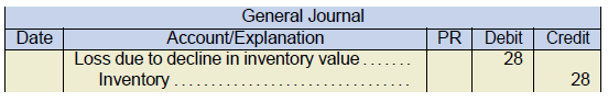
Description Category Cost ($) Selling Price LCNRV Brake pad #1 Brake pads 159 140 140 Brake pad #2 Brake pads 175 180 175 Total brake pads 334 320 315 Soft tire Tires 325 337 325 Hard tire Tires 312 303 303 Total tires 637 640 628 Total LCNRV = (315 + 628) = 943
Current carrying value = ($334 + 637) = 971
Adjustment required = (943 − 971) = (28)
Journal entry required:
- With grouping
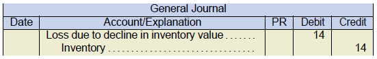
Description Category Cost ($) Selling Price LCNRV Brake pad #1 Brake pads 159 140 Brake pad #2 Brake pads 175 180 Total brake pads 334 320 320 Soft tire Tires 325 337 Hard tire Tires 312 303 Total tires 637 640 637 Only the brake pad category needs to be written down.
Total adjustment required = (320 − 334) = 14
Journal entry required:
Exercise 7.7
NOTE: Positive amounts represent overstatements and negative amounts represent understatements.
| Item | Inventory | A/R | A/P | Net Income |
|---|---|---|---|---|
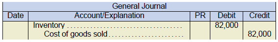
| A | (82,000) | – | (82,000) | |
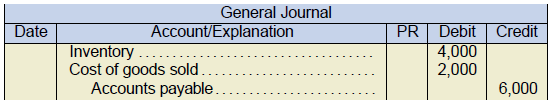
| B | (4,000) | – | (6,000) | 2,000 |
| C | (27,000) | – | – | (27,000) |
| D | (2,000) | 3,500 | – | 1,500 |
| Total | (115,000) | 3,500 | (6,000) | (105,500) |
Exercise 7.8
-
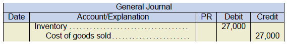
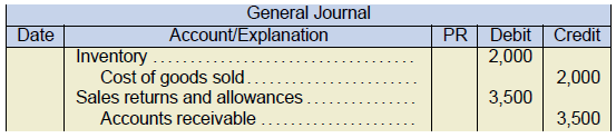
- The journal entries would be the same, except any income statement accounts (cost of goods sold and sales returns) would be replaced with an adjustment to retained earnings.
Exercise 7.9
Inventory on January 1
Purchases (net of returns)
Goods available for sale
Sales
Less gross profit (35% × $955,000)
Estimated cost of goods sold
Estimated inventory on March 4
Less undamaged goods (90,000 × (1 − 0.35))
Inventory damaged by fire
$955,000
334,250
$ 275,000
634,000
909,000
620,750
288,250
(58,500)
$ 229,750
Exercise 7.10
Gross profit margin, by year:
2020: 3,058 ÷ 20,722 = 14.76%
2019: 2,831 ÷ 13,972 = 20.26%
The company’s sales increased significantly between 2019 and 2020. This appears to be a positive result. The company’s gross profit also increased. However, the gross profit margin decreased by 5.5%, which represents potential loss profits of approximately $1.1 billion on the current sales volume. To investigate further, one should look at budgets and other management plans, as well as industry averages and competitor information. It would also be useful to look at longer trends to see if this decline in profitability is unique to this year or the sign of a longer term trend. Management explanations of the declining margin percentage, contained in the annual report, should also be evaluated to determine if the causes relate to slashing sales prices to increase volumes, increasing cost structures, or some combination of the two. Other macroeconomic data may also be useful in explaining the change.
Inventory Turnover Period, by year:
2020: [(2,982 + 1,564) ÷ 2 ÷ 17,164] × 365 = 48.34 days
2019: [(1,564 + 1,239) ÷ 2 ÷ 11,141] × 365 = 45.91 days
Inventory turnover has slowed from the previous year, indicating that goods are being held longer. This is also indicated by the build up of inventory over the three year period. Although the increased inventory may be reasonable as sales increase, the increase in the turnover period could create cash flow problems if the trend continues. Again, other comparative data is needed, such as budgets and industry averages, to evaluate the meaning of this result.
Exercise 7.11
|
Item |
Cost |
Selling Price |
Disposal Costs |
NRV(1) |
LCNRV |
|---|---|---|---|---|---|
| DWE223 | $1,950 | $2,230 | $99 | $2,131 | $1,950 |
| CWQ103 | 5,120 | 4,960 | 112 | 4,848 | 4,848 |
| BMA112 | 4,280 | 4,615 | 225 | 4,390 | 4,280 |
| AAW102 | 3,965 | 4,430 | 91 | 4,339 | 3,965 |
| $15,315 | $15,043 | ||||
| NRV(1) = net realizable value (selling price - disposal costs) | |||||
Adjustment needed for inventory:
| Cost | $15,315 | ||
| LCNRV | $15,043 | ||
| decrease: | $272 | ||
| Loss due to decline in inventory value | 272 | ||
| Inventory | 272 | ||
| ***NOTE - cost of goods sold can be used (direct write off) | |||
Exercise 7.12
| Dec 31, Y5 | Loss on Purcahse Contract | 399,300 | ||
| Liability for Onerous Contract | 399,300 | |||
| the decrease in value should be recorded ($3,456,900 - $3,057,600) | ||||
| Y6 - possession | Purchases | 3,057,600 | ||
| Liability for Onerous Contract | 399,300 | |||
| Accounts Payable | 3,456,900 | |||
| In Y6 - when the contract is satisfied and Highbury takes possession of the items the amount of the agreed upon liability has to be recorded. | ||||
| However, the items are only worth $3,057,600 which is the current, market value. | ||||
| With IFRS, we only record potential losses, not gains (Conservatism). | ||||
| Y6 - payment | Accounts Payable | 3,456,900 | ||
| Cash | 3,456,900 | |||
Exercise 7.13
1. Gross margin method
| Beginning inventory (at cost) | 135,460 | |
| Purchases (at cost) | 2,569,840 | |
| Goods available for sale | 2,705,300 | |
| Sales (actual @ selling price) | 3,156,900 | |
| Less Gross profit (30% of sales) | 947,070 | |
| Sales (at cost) | 2,209,830 | |
| Estimated ending inventory | $495,470 |
2. Determine the markup – to estimate inventory
| First, gross profit as a percent of sales must be calculated | |||
|
30%
(100% + 30%)
|
23.08% | ||
| Beginning inventory (at cost) | 135,460 | ||
| Purchases (at cost) | 2,569,840 | ||
| Goods available for sale | 2,705,300 | ||
| Sales (actual @ selling price) | 3,156,900 | ||
| Less Gross profit (23.08% of sales) | 728,515 | ||
| Sales (at cost) | 2,428,385 | ||
| Estimated ending inventory | $276,915 | ||
| If cost of sales = | 2,428,385 | ||
| 30% markup = | 728,515 | (cost of sales × 30% = $2,428,385 × 30%) | |
| Sales (actual @ selling price) | 3,156,900 | ||
| Or - $3,156,900 / 1.30 | 2,428,385 | (is the cost) | |
Exercise 7.14
1. Ending inventory overstated
| 1. Working capital | Overstated by $5,300 |
| 2. Current ratio | Overstated |
| 3. Retained earnings | Overstated by $5,300 |
| 4. Net income | Overstated by $5,300 |
2. Purchase not recorded
| 1. Working capital | No effect |
| 2. Current ratio | Overstated |
| 3. Retained earnings | No effect |
| 4. Net income | No effect |
3. Ending inventory and purchases understated
| 1. Working capital | Overstated by $3,890 |
| 2. Current ratio | Overstated |
| 3. Retained earnings | Overstated by $3,890 |
| 4. Net income | Overstated by $3,890 |
