7.3 Subsequent Recognition and Measurement

Once the initial inventory amounts have been determined and recorded, a number of subsequent accounting decisions need to be made. These decisions can be summarized in the following questions:

• What type of inventory accounting system should be used?
• What cost flow assumption should be applied?
• What method can be applied to ensure reported inventories are not overvalued?

We will examine each of these issues in the following sections.

7.3.1 Inventory Accounting Systems

A merchandising business can typically be engaged in thousands or millions of inventory transactions each year. As well, inventory can comprise a significant proportion of a merchandising company’s total assets. It is thus important for merchandising businesses to have robust and accurate systems in place for gathering data on inventory transactions. The use of various technologies, such as computers, bar codes, and RFIDs, has simplified the complex task of gathering inventory transaction information. The use of such technologies has allowed most businesses to implement perpetual inventory systems as their data-collection method. A perpetual inventory system is one that tracks all inventory additions and subtractions (purchases and sales) directly in the accounting records. Thus, at any point in time, the company can produce an accurate income statement and balance sheet that will display the amount of the cost of goods sold for the period and inventory balance at the end of the period. This type of system provides more timely information to managers, which can lead to better decision processes.

A periodic inventory system, on the other hand, does not track purchases and sales of inventory items directly in the accounting records. Rather, purchases are tracked through a separate purchases account, and the cost of goods sold is not recorded at all at the time of sale. The cost of goods sold can be determined only at the end of the accounting period, when a physical inventory count is taken, and the ending inventory is then reconciled with the opening inventory. This type of system is less useful for management purposes, as profitability can be determined only at the end of the accounting period. As well, the balance sheet would not reflect the appropriate inventory balance until the period-end reconciliation is performed. Periodic inventory systems may be appropriate for a small business where accounting resources are limited, but improvements in technology have resulted in many businesses switching to perpetual inventory systems.

Note that although a perpetual inventory system does result in an instantaneous update of inventory accounts, physical inventory counts are still required under this system. There are many situations, such as product spoilage or theft, that are not captured by perpetual inventory systems, so it is important that companies employing these systems still physically verify the goods at least once per year.

7.3.2 Cost Flow Assumptions

The issue of cost flow assumptions can become particularly important when prices of inventory inputs are changing. Consider a merchandising company that purchases inventory items on a continuous basis in order to fill customer orders. At any given point during the accounting period, the goods available for sale may consist of identical items that were purchased at different times for different costs. The question the accountant must answer is, which costs should be allocated to the current cost of goods sold and which costs should continue to be held in inventory? To answer this question, the accountant can choose from three possible methods:

• Specific identification
• Average cost (moving average and weighted average)
• First in, first out

Specific Identification

This technique is theoretically the most correct way to allocate costs. Each unit that is sold is specifically identified, and the cost for that unit is allocated to cost of goods sold. This method would thus achieve the perfect matching of costs to the revenue generated. There are, however, some disadvantages to this method. First, unless items are easy to physically segregate, it may difficult to identify which items were actually sold. As well, although physical segregation may be possible, this method could be expensive to implement, as a great deal of record keeping is required.

The second disadvantage of this method is its susceptibility to earnings-management techniques. If a manager wanted to manipulate the current period net income, he or she could do this very easily using this method by simply choosing which items to sell and which to retain in inventory. Lower cost items could be shipped to customers, which would result in lower cost of goods sold, higher profits, and higher inventory values on the statement of financial position. Because of this potential problem, this technique should be applied only in situations where inventory items are not normally interchangeable with each other. An example of this would be the inventory held by a car dealership. Each item would have a separate serial number and could not be substituted for another item.

Average Cost

This technique can be applied to either periodic or perpetual inventory systems by calculating the average of all goods available for sale and then allocating the average to both the quantity of goods sold and the quantity of goods retained in inventory. When this technique is applied to a perpetual inventory system, it is usually referred to as a moving average cost. An example of a moving average cost calculation is as follows:

The following transactions occurred in the month of May for PartsPeople Inc.

Date	Transaction
May 1	Opening inventory	300 units @ $3.00
May 3	Purchase	100 units @ $3.20
May 7	Purchase	200 units @ $ 3.25
May 11	Sale	150 units
May 22	Purchase	250 units @ $3.30
May 25	Sale	375 units
May 31	Ending inventory	325 units

Inventory and cost of goods sold would be calculated as follows:

Date	Purchase	Cost of Goods Sold	Balance	Moving Average[1]	Balance of Units
May 1			300 × $3.00 = $900.00	$3.0000	300
May 3	100 × $3.20		(300 × $3.00) + (100 × $3.20) = $1,220.00	$3.0500	400
May 7	200 × $3.25		(300 × $3.00) + (100 × $3.20) + (200 × $3.25) = $1,870.00	$3.1167	600
May 11		150 × $3.1167 = $467.50	450 × $4.1167 = $1,402.50	$3.1167	450
May 22	250 × $3.30		(450 × $3.1167) + (250 × $3.30) = $2,227.50	$4.1821	700
May 25		375 × $3.1821 = $1,193.30	325 × $3.1821 = $1,034.20	$3.1821	325

The total cost of goods sold for the period is ($467.50 + $1,193.30) = $1,660.80, and the ending inventory balance is $1,034.20. Under this approach, the average inventory cost is recalculated after each purchase, and this revised average cost is then used to determine the cost of goods sold when a sale is made. After a sale is made, the revised average cost becomes the new base amount for further inventory transactions until the next purchase occurs, and a new average is determined.

This method is often used due to its simplicity and reliability. It is very difficult for managers to manipulate income with this method, as the effects of rising or falling prices will be averaged over both the goods sold and the goods remaining on the balance sheet. As well, for goods that are similar and interchangeable, this method may most closely represent the actual physical flow of those goods.

A somewhat easier average cost method of determining inventory and cost of goods sold is the weighted average. As the name implies, an average cost method prices inventory items based on the average of the purchases in order to determine an average cost of goods sold. The weighted average method takes into account that the value of each purchase is different.

The following transactions occurred in the month of May for PartsPeople Inc.

Date	Transactions
May 1	Opening inventory	300 units @ $3.00
May 3	Purchase	100 units @ $3.20
May 7	Purchase	200 units @ $3.25
May 11	Sale	150 units
May 22	Purchase	250 units @ $3.30
May 25	Sale	375 units
May 31	Ending inventory	325 units

With the weighted average method, we only consider the goods that are available for sale. That means the beginning inventory and the purchases are included in order to determine a weighted average cost per unit.

Date	Transactions
May 1	Opening inventory	300 units @ $3.00 = $900
May 3	Purchase	100 units @ $3.20 = $320
May 7	Purchase	200 units @ $3.25 = $650
May 22	Purchase	250 units @ $3.30 = $825
	Total	850 units = $2,695

Weighted average cost per unit = $2,695850 units = $3.17/unit.

The cost of the ending inventory is 325 units × $3.17 = $1,030.25

The cost of goods sold is equal to the number of units sold (150 units + 375 units) = 525 units multiplied by the weighted average cost per unit or, 525 units × $3.17 = $1,664.25.

First in, First out (FIFO)

Another cost-flow choice companies can use is referred to as the first in, first out method, usually abbreviated as FIFO. This method allocates the oldest costs to goods sold first, with newer costs remaining in the inventory balance. Assume the same set of facts for PartsPeople Inc. used in the previous example. Under FIFO, each time a sale occurs, the oldest items are removed from inventory first. The calculation of costs and inventory amounts would be done as follows:

Date	Purchase	Cost of Goods Sold	Balance	Balance of Units
May 1			300 × $3.00 = $900.00	300
May 3	100 × $3.20		(300 × $3.00) + (100 × $3.20) = $1,220.00	400
May 7	200 × $3.25		(300 × $3.00) + (100 × $3.20) + (200 × $3.25) = $1,870.00	600
May 11		150 × $3.00 = $450.00	(150 × $3.00) + (100 × $3.20) + (200 × $3.25) = $1,402.00	450
May 22	250 × $3.30		(150 × $3.00) + (100 × $3.20) + (200 × $3.25) + (250 × $3.30) = $2,245.00	700
May 25		(150 × $3.00) + (100 × $3.20) + 125 × $3.25) = $1,176.25	(75 × $3.25) + (250 × $3.30) = $1,068.75	325

In this case, the total ending inventory balance of $1,068.75 is higher than the balance calculated under the moving average cost system. This makes sense, as FIFO inventory balances represent the most recent purchases, and in this scenario, input costs were rising throughout the month. This feature of FIFO is considered one of its strengths, as the method results in balance-sheet amounts that more closely represent the current replacement cost of the inventory. Also note that the total cost of goods sold of $1,626.25 ($450.00 + $1,176.25) is lower than moving average amount. This also makes sense, as older costs, which are lower in this case, are being expensed first. This characteristic of FIFO is also one of its major drawbacks. The method of expensing older costs first means that proper matching is not being achieved, as current revenues are being matched to older costs. This method thus represents a trade-off common in accounting standards. A more relevant balance sheet results in a less relevant income statement. Moving average, on the other hand, averages out the differences between the balance sheet and income statement, resulting in some loss of relevance for both statements. As both methods are acceptable under IFRS and ASPE, management would have to decide which statement is more important to the end users and then choose a policy accordingly.

How to Choose?

When making an inventory cost flow assumption, what factors do managers need to consider? Generally, the cost flow assumption should attempt to reflect the actual physical flow of goods as much as possible. For example, a grocery retailer selling perishable merchandise may want to use FIFO, as it is common practice to place the oldest items at the front of the rack to encourage their sale first. Alternatively, consider a hardware store that sells bulk nails that are scooped from a bin. There is no way to identify the individual items specifically, and it is likely that over time, customers scooping out nails would mix together items stocked at different times. Weighted average costing would make the most sense in this case, as this would likely represent the real movement of the product. For a company selling heavy equipment, specific identification would likely make the most sense, as each item would be unique with its own serial number, and these items can be easily tracked.

A further consideration would be the effects on the income statement and balance sheet. FIFO results in the inventory reported on the balance being reported at more current costs. As there is an increasing emphasis in standard setting on valuation concepts, this approach would result in the most useful information for determining the value of the company. If profitability is more important to a financial-statement reader, then weighted average cost would be more useful, as more current costs would be averaged into income.

Income taxes may also be a consideration when choosing a cost flow formula. This motivation must be considered carefully, however, as income will be affected in opposite ways, depending on whether input prices are rising or falling. As well, although taxes could be reduced in any given year through the cost flow assumption made, this is only a temporary effect, as all inventory will eventually be expensed through cost of goods sold.

Whatever method is chosen, it should be applied on a consistent basis. It would be inappropriate for a company to change cost flow assumptions year to year, simply to achieve a certain result in net income. Once the cost flow assumption is determined, it should be applied the same way each year, unless there has been a significant change in circumstances that warrants a change. A company may use different cost flow assumptions for different major inventory classes, but these choices should still be applied consistently.

As a historical note, a further cost flow assumption, last in, first out (LIFO), was once available for use. This method took the most recent purchases and allocated them to the cost of the goods sold first. LIFO is now not allowed in Canada under IFRS or ASPE, but it is still used in the United States. Although this method resulted in the most precise matching on the income statement, tax authorities criticized it as way to reduce taxes during periods of inflation. As well, it was more easily manipulated by management and did not result in accurate valuations on the balance sheet. Canadian companies that are allowed to report under US GAAP may still use this method, but it is not allowed for tax purposes in Canada.

7.3.3 The Problem of Overvaluation

Overvaluation can occur when inventory is reported at a higher value than the ultimate amount that can be recovered. This happens with changes in market conditions or consumer tastes, or it happens for other reasons. If a particular product loses favour with the market and must be severely discounted or even disposed of, it would not be appropriate to continue to carry that item on the balance sheet at its cost when that cost is not recoverable. To avoid this problem, the lower of cost and net realizable value (LCNRV) needs to be applied. This method is sometimes also referred to as the lower of cost or market (LCM). Under this approach, inventory values are reduced to their recoverable amounts in order to ensure that current assets are not stated at an amount greater than the ultimate amount of cash that will be realized from their sale. This also results in recording an expense equal to the loss in value of the asset, which achieves the effect of matching the cost to the period in which the loss actually occurs. For example, if an inventory item has a reported cost of $1,000 but a net realizable value of only $800, the company should record the following journal entry:

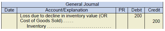
Most companies will simply report the loss (adjustment) as part of the cost of goods sold account on the income statement. Separate disclosure may be appropriate, however, if the amount is considered material or unusual in nature.

What Is Net Realizable Value?

When determining the loss in inventory value, it is important to have a clear understanding of the concept of net realizable value (NRV). Net realizable value is an estimate based on the expected selling price of the goods in the ordinary course of business, less any estimated costs required to complete and sell the goods. It thus represents the net cash flow that will ultimately be generated by the sale of the product. Because the net realizable value is an estimate, it can be affected by management estimation bias and by changes in economic circumstances. As a result, write-downs of inventories need to be reviewed carefully and frequently by accountants to ensure the reported amounts are reasonable.

How Is the Lower of Cost and Net Realizable Test Applied?

In general, the lower of cost and net realizable test should be applied to the most detailed level possible. This would normally be considered to be individual inventory items. However, in some situations, it may be appropriate to group inventory items together and apply the test at the group level. This would be appropriate only when items relate to the same product line, have similar end uses, are produced and marketed in the same geographic area, and cannot be segregated from other items in the product line in a reasonable or cost-effective way. If grouping is appropriate, the amount of inventory write-downs will be less than if the test is applied on an individual-item basis. This occurs because grouping allows for some offsetting of over- and undervalued items.

In summary, the lower or cost and net realizable value method requires that inventory be valued at cost unless the net realizable value is lower than cost. If NRV is lower than cost, the inventory should be value at the NRV.

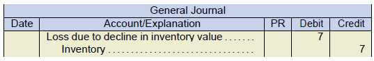
To apply the method:

1. Determine the cost.
2. Calculate the net realizable value (selling price less costs to sell).
3. Compare the two items (cost and net realizable value).
4. Chose the lower value of the two items.

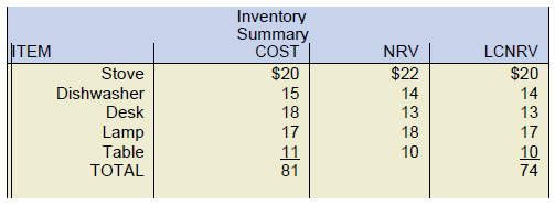
From the above table, the LCNRV is less than cost; therefore,an adjustment should be made to properly reflect the value of the inventory. If the LCNRV would have been greater than the cost, no adjustment would be made and inventory would be properly reflected at the lower amount – the cost.

Purchase Commitments

Some businesses may find the need to buy inventory items weeks or months in advance of using the item. These purchases are agreed to based on estimated sales commitments determined by the company’s customers. Title to the goods or services from these purchase commitments does not pass to the buyer until delivery of the good or service is made. It’s important to realize that when a commitment is made, the good may not even exist. However, a commitment (contract) may be set with a price of the items agreed to purchase.

IFRS rules apply when there is a potential onerous contract. This means that if there are unavoidable costs of satisfying the contract that are higher than the expected benefits from receiving the agreed amount of goods or services, a loss provision can be recognized.

As an example:

Suppose a company signs several purchase commitments. Under the terms of one of the commitment, the company will take delivery of the inventory in the following year. The agreed upon price is $830,000. Now suppose that the fair value of these items declines to $550,000 at the companies fiscal year. The company does not expect to recover any additional costs. Assume that the fair value of the items remains at the reduced fair value of $550,000 until the items are delivered.

Is this an onerous contract? What are the entries?

This contract has become onerous because of the reduction in the fair value of the goods.

At the time of the contract signing, there is NO journal entry. It is a contract and an agreement but no journal entry is required when the contract has been signed since nothing has changed hands.

At the time the contract is considered onerous (the fiscal year end in this example):

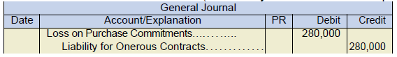
The amount is determined by taking the difference between the agreed upon price of $830,000 and the fair value of $550,000. ($830,000 − $550,000 = $280,000).

When the goods are received:

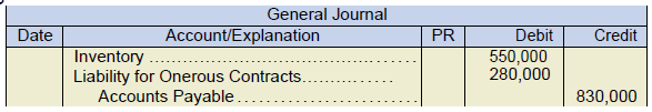
It’s important to note that the company would still owe the amount agreed upon ($830,000). Also note that if the price of the items had partially or fully recovered to the agreed upon amount, the Liability for Onerous Contracts would be reduced.

Biological Assets

One interesting exception to the lower of cost and net realizable value rule is accounting for biological assets. Although ASPE does not specifically address these types of assets, IFRS does present a separate standard: IAS 41 Agriculture. This standard covers raising and harvesting living plants and animals. The biological assets are considered the original source of the commercial activity, such as the fruit tree that produces apples, the sheep that produces wool, or the dairy cow that produces milk. The detailed accounting for these specialized assets goes beyond the scope of this course.

Generally, the product of the biological asset would fall under the normal rules for inventory accounting, but the biological asset itself is accounted for at its fair value, less selling costs. This means that every year, the value of the biological-asset must be determined, and an adjustment to the assets carrying value must be made. This adjustment would result in an unrealized gain or loss. As the inventory is produced, it is transferred from the biological-asset account to an inventory account at its fair value less selling costs at the point of harvest. This value now becomes the inventory’s cost. When inventory is sold, the sale amount is transferred from the unrealized account to realized revenue.

Conceptually, these types of assets are similar in nature to a capital asset, but they are also different in that they grow and obtain value independent of the inventory they produce. This unique nature is the reason IFRS presents a separate standard for the accounting and disclosure of biological assets.