6.3 Receivables
Receivables are asset accounts applicable to all amounts owing, unsettled transactions, or other monetary obligations owed to a company by its credit customers or debtors. In general, receivables are claims that a company has against customers and others, usually for specific cash receipts in the future. These are contractual rights that have future benefits such as future cash flows to the company. These accounts can be classified as either a current asset, if the company expects them to be realized within one year or as a long-term asset, if longer than one year. Receivables are initially valued at their fair value (at time of sale).
Typical receivable-related categories include:
- Accounts (trade) receivable—amounts owed by customers for goods or services sold by a company on credit in the normal course of business. The transaction document is typically called an invoice. An important note – some companies may use the term “accounts” receivable while others use the term “trade” receivables. Both terms are acceptable. It’s also important to note that often, accounts receivable are reported at “net”. Net receivables (or net realizable value) are equal to the accounts receivable amount less any allowance for doubtful accounts (discussed later in this chapter).
- Notes receivable—more formal, unconditional written promises to pay a specified amount of money on a specified future date or on demand. Usually, these documents are in writing and are therefore more formal. The transaction document is usually referred to as a promissory note.
- Non-trade receivable—arise from any number of other sources such as income tax refunds, GST/HST taxes receivable, amounts due from the sale of assets, insurance claims, advances to employees, amounts due from officers, and dividends receivable. These are generally classified and reported as separate items in the balance sheet or in a note that is cross-referenced to the balance sheet statement.
The table below shows a portion of the balance sheet for cash and cash equivalents and various receivables on the financial statements:
| Consolidated Balance Sheet As of December 31, 2020 and 2019 (In millions of dollars except share amounts) |
||
|---|---|---|
| Assets | 20201 | 2021 |
| Cash and cash equivalents | 3,500 | 4,200 |
| Marketable securities | 1,500 | 1,400 |
| Receivables from affiliates | 30 | 60 |
| Trade accounts and notes receivables (net) | 3,800 | 3,800 |
| Financing receivables (net) | 25,500 | 22,200 |
| Financing receivables, securitized (net) | 4,300 | 3,200 |
| Other receivables | 1,000 | 1,500 |
| Operating leases receivables (net) | 3,000 | 2,500 |
Receivables Management
It is important to consider carefully how to manage and control accounts receivable balances. If credit policies are too restrictive, potential sales could be lost to competitors. If credit policies are too flexible, more sales to higher risk customers may occur, resulting in more uncollectible accounts. The bottom line is that receivables management is about finding the right level of receivables to maintain when implementing the company’s credit policies.
As part of a credit assessment process, companies will initially assess the individual creditworthiness of new customers and grant them a credit limit consistent with the level of assessed credit risk. After the initial assessment, a customer’s payment history will affect whether their credit limit will change or be revoked.
To lessen the risk of uncollectible accounts and improve cash flows, some companies will adopt a policy that offers:
- Cash discounts to encourage cash sales
- Sales discounts to encourage faster payments of amounts owing on credit
- Late payment interest charges for any overdue accounts
Other management strategies can be implemented to shorten the receivables to cash cycle. In addition to the discounts or late payment fees listed above, small- and medium- sized companies may decide to sell their accounts receivable to financial intermediaries (factors). This will convert the receivables into cash more quickly than if they waited for customers to pay. Larger companies may rely on another way of selling receivables, called securitization. This will be discussed later in this chapter.
Receivables management involves developing sound business practices for overall monitoring as well as early detection of potential uncollectible accounts. Key activities include:
- Regular analysis of aged accounts receivable
- Regularly scheduled assessments and follow up on overdue accounts
6.3.1. Accounts Receivable
Recognition and Measurement of Accounts Receivable
Accounts receivable result from credit sales in the normal course of business (called trade receivables) that are expected to be collected within one year. For this reason, they are classified as current receivables on the balance sheet and initially measured at the time of the credit sale at their net realizable value (NRV). Net realizable value (NRV) is the amount expected to be received from the customer. IFRS and ASPE standards both allow NRV to approximate the fair value, since the interest component is immaterial when determining the present value of cash flows for short-term accounts receivable. In subsequent accounting periods, accounts receivable are to be measured at their amortized cost which is the same as cost, since there is no present value interest component to recognize. For long-term notes and loans receivable that have an interest component, the asset’s carrying amount is measured at amortized cost which will be described later in this chapter.
The valuation of the account receivable is also affected by:
- Trade and sales discounts
- Sales returns and allowances
Trade Discounts
Manufacturers and wholesalers publish catalogues with inventory and sales prices to assist purchasers with their purchases. Catalogues are expensive to publish, so this is only done from time to time. Sellers often offer trade discounts to customers to adjust the sales prices of items listed in the catalogue. This can be an incentive to purchase larger quantities, as a benefit of being a preferred customer or because costs to produce the items for sale have changed.
Since the catalogue, or list, price is not intended to reflect the actual selling price, the seller records the net amount after the trade discount is applied. For example, if a plumbing manufacturer has a catalogue or list price of $1000 for a bathtub and sells it to a plumbing retailer for list price less a 20% trade discount, the sale and corresponding account receivable recorded by the manufacturer is $800 per bathtub.
Sales Discounts
Sales discounts can be part of the credit terms for customers and are offered to encourage faster payment of the account. The credit term 1.5/10, n/30 means there is a 1.5% discount if the invoice is paid within ten days with the total amount owed due in thirty days.
Companies purchasing goods and services that do not take advantage of the sales dis- counts are usually not using their cash as effectively as they could. For example, a purchaser who fails to take the 1.5% reduction offered for payment within ten days for an account due in thirty days is equivalent to missing a stated annual interest rate return on their cash for 27.38% (365 days ÷ 20 days × 1.5%). For this reason, companies usually pay within the discount period unless their available cash is insufficient to take advantage of the opportunity.
IFRS 15.53 – the term variable consideration, discussed in Chapter 5, Revenue, would also include sales discounts because it is uncertain how many customers will actually take the sales discount. For this reason, IFRS states that an estimate of “highly probable” sales discounts expected to be taken by customers, needs to be determined and included at the time of the sale. Given the high rate of return identified in the preceding paragraph, recording the estimate immediately upon sale is conceptually sound and is consistent with the net method described below. The standard suggests using either the expected value (a weighted average of probabilities), or the “most likely amount” to estimate sales discounts, perhaps based on past history.
To illustrate the net method, assume that Cramer Plumbing sells fifty bathtubs to a reseller for $800 each, for a total sale of $40,000, with credit terms of 1.5/10, n/30. Using the net method, Cramer expects that the sales discount will be taken by the purchaser; therefore, Cramer Plumbing will record the following entry:
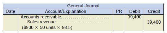
Note the reduction due to the sales discount is immediately recorded upon the sale. This results in the accounts receivable being valued at its net realizable value and based on Cramer’s “more likely than not” estimate of sales discounts expected to be taken, which is consistent with IFRS 15.53.
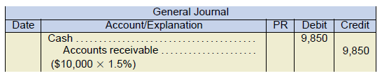
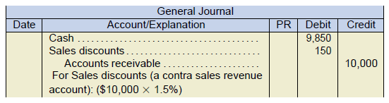
If $10,000 of the account receivable is collected from the reseller within the ten-day discount period (for a cash amount of $9,850), the entry would be:
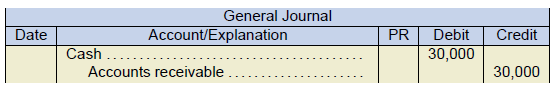
The entry for collection of the remaining amount owing for $30,000 after the discount period is:
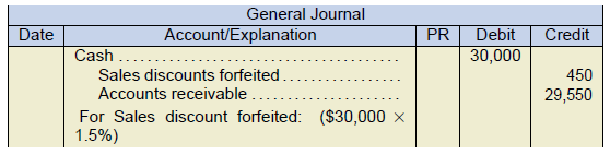
As can be seen above, the net method records and values the accounts receivable at its lowest, or net realizable value of $39,400, or gross sales for $40,000 less the 1.5% discount.
The gross method is much easier and ASPE can choose either method. For the gross method, sales are recorded at the gross amount with no discount taken. If the customer pays within the discount period, the applicable discount taken is recorded to a sales discounts account. Any payments made after the discount period are simply the cash amount collected and no calculation for the sales discounts forfeited is required.
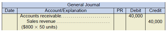
Using the same example, assume that Cramer Plumbing sells fifty bathtubs for $800 each, with credit terms of 1.5/10, n/30. Using the gross method, the entry for the sale is:
The entry on collection of $10,000 within the ten-day discount period is:
The entry on collection of the remaining $30,000 after the discount period is:
Note how the accounts receivable would not be reported at its net realizable value with this method. If discounts are significant, this would overstate accounts receivable and sales in the financial statements. For this reason, if the gross method is used and it is expected that significant cash discounts are likely to be taken by customers in the fiscal year, an asset valuation account and an adjusting entry is required to ensure that accounts receivable, net of the valuation account, will reflect its net realizable value.
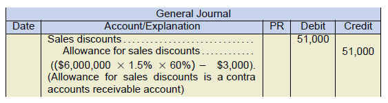
At year-end, assume that $6 million of Cramer’s accounts receivable all have terms of 1.5/10, n/30, and management expects that 60% of these accounts will be collected within the discount period, which it deems to be significant. The unadjusted balance in the allowance for sales discounts account (a contra account to accounts receivable) is $3,000 credit balance. The year-end adjusting entry to update the accounts receivable allowance account with the estimated sales discounts would be:
Throughout the following year, the allowance account can be directly debited each time customers take the discounts and is adjusted up or down at the end of each reporting period.
Sales Returns and Allowances
Many ASPE companies have policies that allow for the return of goods under certain circumstances and will refund all or a partial amount of the returned item’s cost.
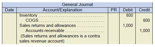
Assuming that returns for this company are insignificant, the entry for a $1,000 sales return on account (with a cost $800) returned to inventory, for a company using a perpetual inventory system, would be:
Sales allowances are reductions in the selling price for goods sold to customers, perhaps due to damaged goods that the customer is willing to keep if the sales price is reduced sufficiently. On the income statement, sales returns and allowances would reduce sales.
For example, if a sales allowance of $2,000 is granted due to damaged goods that the customer chose to keep, the entry, assuming sales allowances for this company are insignificant, would be:
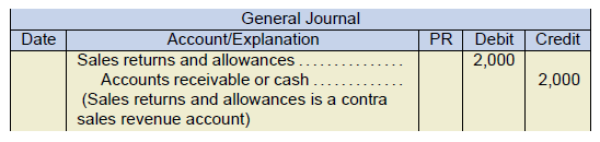
As was done with sales discounts, sales returns and allowances should be recognized in the period of the sale to avoid overstating accounts receivable and sales. Sales returns and allowances are therefore estimated and adjusted at the end of each reporting period. If the amount of returns and allowances is not material a year-end adjusting entry is not required and the entries shown above would be sufficient, provided that it is handled consistently from year to year. If returns and allowances are significant, an allowance for sales returns and allowances account, which is an asset valuation account contra to accounts receivable, is used to record the estimates.
For example, management estimates the total sales returns and allowances to be $51,500, which it deems to be significant. If the company follows ASPE, and the unadjusted balance in the allowance for sales returns and allowances account is $5,000 credit balance, the year-end adjusting entry would be:
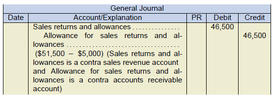
Note how another contra account, the sales returns and allowances account, is used to record the debit entry for the previous two journal entries above. Its purpose is to track returns and allowances transactions separately, as opposed to directly recording them as a debit to sales. If amounts in this contra account become too high, it could indicate to management the possibility of future sales lost due to unsatisfied customers.
During the reporting period, the allowance for sales returns and allowances asset valuation account can be directly debited each time customers are granted returns or allowances. This asset valuation account will subsequently be adjusted up or down at the end of each reporting period.
Sales with right of return under IFRS has been discussed in Section 5.3.3, Sales With Right of Return, where a detailed example is presented.
Estimating Allowance for Uncollectible Accounts (Impairment)
When accounts receivables exist, some amounts of uncollectible receivables are inevitable due to credit risk. This risk is the likelihood of loss due to customers not paying their amounts owing. If the uncollectible amounts are both likely and can be estimated, an amount for uncollectible accounts must be estimated and recognized in the accounts to ensure that accounts receivable and net income are not overstated over the lifetime of the accounts receivable (IFRS 9; lifetime expected credit losses). The allowance account, called the allowance for doubtful accounts (AFDA), is an asset valuation account (contra account to accounts receivable), which is used the same way as the Allowance for Sales Discounts discussed earlier.
Many companies set their credit policies to allow for a certain percentage of uncollectible accounts. This is to ensure that the credit policy is not too restrictive or liberal, as explained in the opening paragraph of the Receivables Management section of this chapter.
Measuring uncollectible amounts at the end of each reporting period involves estimates that can be calculated using several methods:
- Percentage of accounts receivable method
- Accounts receivable aging method
- Credit sales method
- Mix of methods
The first three methods were covered in the introductory accounting course. Below is a review of these methods. The mix of methods is perhaps a more realistic view of how companies estimate bad debt expense over a reporting period.
For each method above, management estimates a percentage that will represent the likelihood of collectability. The estimated total amount of uncollectible accounts is calculated and usually recorded to the AFDA allowance account, with the offsetting entry to bad debt expense. The net amount for accounts receivable and its contra account, the AFDA, reflects the net realizable value of the accounts receivable at the reporting date.
Percentage of Accounts Receivable Method
For this method, the accounts receivable closing balance is multiplied by the percentage that management estimates is uncollectible. This method is based on the premise that some portion of accounts receivable will be uncollectible, and management uses reasonably available and supportable information (IFRS 9) regarding past experiences, current economic conditions, and expected future conditions as a guide to the percentage used. For this reason, the estimated amount of uncollectible accounts is to be equal to the adjusted ending balance of the AFDA. The adjusting entry amount must therefore be the amount required that results in that ending balance of the AFDA.
For example, assume that accounts receivable and the AFDA ending balances were $200,000 debit and $2,500 credit balances respectively at December 31, and the uncollectible accounts is estimated to be 4% of accounts receivable. This means that the AFDA adjusted ending balance is estimated to be the amount equal to 4% of $200,000, or $8,000. The adjusting entry to achieve the correct AFDA adjusted ending balance of $8,000 would be:
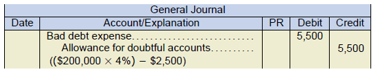
The AFDA ending balance after the adjusting entry would correctly be $8,000 ($2,500 unadjusted balance + $5,500 adjusting entry).
![]() REMEMBER– AFDA normally should have a credit balance.
REMEMBER– AFDA normally should have a credit balance.
Sometimes the AFDA ending balance can be in a temporary debit balance due to a write-off of an uncollectible account during the period. If this is the case, care must be taken to make the correct calculations for the adjusting entry. For the example above, if the unadjusted AFDA balance was a $300 debit balance, then the adjusting entry for uncollectible accounts would be:
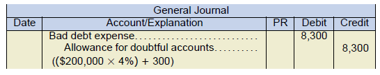
The AFDA ending balance after the adjusting entry would correctly be $8,000 ($300 debit + $8,300 credit).
Notice that the AFDA ending balance of $8,000 is the same for both examples when applying the percentage of accounts receivable method. This is because the calculation is intended to be an estimate of the AFDA ending balance, so the adjustment amount is whatever is required to result in that ending balance.
Accounts Receivable Aging Method
Typically, the older the uncollected account, the more likely it is to be uncollectible. Fol- lowing this premise, the accounts receivable are grouped into categories based on the length of time they have been outstanding.
Just as was done for the percentage of accounts receivable method above, companies will use past experience to estimate the percentage of their outstanding receivables that will become uncollectible for each aged group, such as the four aging groups identified in the schedule below. The sum of all the estimated uncollectible amounts by group represents the total estimated uncollectible accounts. Just like the percentage of accounts receivable method previously discussed, the estimated amount of uncollectible accounts using this method is to be equal to the ending balance of the AFDA account . The adjusting entry amount must therefore be whatever amount is required to result in this ending balance.
Aging schedules are also a good indicator of which accounts may need additional attention by management, due to their higher credit risk group, such as the length of time the account has been outstanding or overdue.
Below is an example of an accounts receivable aging schedule:
| Taylor and Company Aging Schedule As at December 31, 2020 |
|||||
|---|---|---|---|---|---|
| Customer | Balance Dec 31, 2020 |
Under 60 day | 61-90 days | 91-120 days | Over 120 days |
| Abigail Holdings | $3,500 | $1,500 | $2,000 | ||
| Beaver Industries Inc. | 45,000 | 25,000 | 8,500 | $6,500 | $5,000 |
| Cambridge Instruments Co. | 18,000 | 18,000 | |||
| Dereck Station Ltd. | 25,000 | 25,000 | |||
| Falling Gate Repair | 6,840 | 6,840 | |||
| Gladstone Walkways Corp. | 26,000 | 26,000 | |||
| : | : | : | . | ||
| Tremsol Cladding Inc. | 15,000 | 10,000 | 4,000 | 1,000 | |
| Warbling Water Pond Installations | 6,480 | 1,480 | 5,000 | ||
| $186,480 | $124,050 | $22,300 | $22,130 | $18,000 | |
| Percent estimated uncollectible | 5% | 10% | 15% | 35% | |
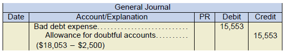
| Total Allowance for uncollectible accounts ending balance | $18,053 | $6,203 | $2,230 | $3,320 | $6,300 |
The analysis above indicates that Taylor and Company expects to receive $186,480 less $18,053, or $168,427 net cash receipts from the December 31 amounts owed. The $168,427 represents the company’s estimated net realizable value of its accounts receivable and this amount would be reported as the net accounts receivable in the balance sheet as at December 31.
Assuming the data above for Taylor and Company and an unadjusted AFDA credit balance as at December 31 of $2,500, the adjusting entry for uncollectible accounts would be:
As was illustrated for the percentage of accounts receivable method above, the calculation of the adjusting entry amount must consider whether the unadjusted AFDA balance is a debit or credit amount.
Remember – AFDA normally has a credit balance. It’s sometimes helpful to use a “T” account when determining the proper allowance amount.
Credit Sales Method
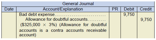
This is the easiest method to apply (and it best illustrates the matching principle). The amount of credit sales (or total sales, if credit sales are not determinable) is multiplied by the percentage that management estimates is uncollectible. Factors to consider when determining the percentage amount to use will be trends resulting from amounts of uncollectible accounts in proportion to credit sales experienced in the past. The resulting amount is credited to the AFDA account and debited to bad debt expense.
Note that for this method, the previous balance in the AFDA account is not taken into consideration. This is because the credit sales method is intended to calculate the bad debt expense that will be reported on the income statement. This is a fast and simple way to estimate bad debt expense because the amount of sales (or preferably credit sales) is known and readily available. This method also illustrates proper matching of expenses with revenues earned over that reporting period. Remember, just use credit sales, watch for any indication of cash sales.
For example, if credit sales were $325,000 at the end of the period and the uncollectible accounts was estimated to be 3% of credit sales, the entry would be:
Mix of Methods
Often companies will use the percentage of credit sales method to adjust the net accounts receivables for interim (monthly) financial reporting purposes because it is easy to apply. At the end of the year, either the percentage of accounts receivable or aging accounts receivable method is used for purposes of preparing the year-end financial statements so that the AFDA account is adjusted accordingly, and reported on the balance sheet.
Below is a partial balance sheet for Taylor and Company using the data from the Accounts Receivable Aging Method section above:
| Taylor and Company Balance Sheet December 31, 2020 |
|
|---|---|
| Current assets: | |
| Accounts receivable | $186,480 |
| Less: Allowance for doubtful accounts | 18,053 |
| $168,427 | |
To summarize, the $186,480 represents the total amount of trade accounts receivables owing from all the credit customers at the reporting date of December 31, 2020. The $18,053 represents the estimated amount of uncollectible accounts calculated using the allowance method, the percentage of sales method, or a mix of methods. The $168,427 represents the net realizable value (NRV) of the receivable at the reporting date.
Write-offs and Collections
Write-off of an Actual Uncollectible Account
Management may deem that a customer’s account is uncollectible and may wish to re- move the account balance from accounts receivable with the offsetting entry to the allowance for doubtful accounts. For example, using the data for Taylor and Company shown under the accounts receivable aging method, assume that management wishes to remove the account for Cambridge Instruments Co. of $18,000 because it remains unpaid despite efforts to collect the account. The entry to remove the account from the accounting records is:
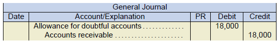
Because the AFDA is a contra account to accounts receivable, and both have been reduced by identical amounts, there is no effect on the net accounts receivable (NRV) on the balance sheet. This treatment and entry makes sense because the estimate for uncollectible accounts adjusting entry (with a debit to bad debt expense) had already been done using one of the allowance methods discussed earlier. The purpose of the write-off entry is to simply remove the account from the accounting records.
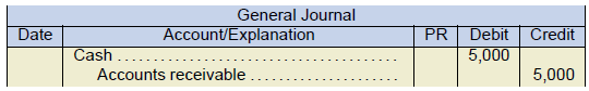
Collection of a Previously Written-off Account
Even though management at Taylor and Company thinks that the collection of the $18,000 account has become unlikely, this does not mean that the company will make no further efforts to collect the amount outstanding from the purchaser. During the tough economic times in 2009 and onward, many companies were in such financial distress that they were simply unable to pay their amounts owing. Many of their accounts had to be written-off by suppliers during that time as companies struggled to survive the crisis. Some of these companies recovered through good management, and cash flows returned. It is important for these companies to rebuild their relationships with suppliers they had previously not paid. So, it is not uncommon for these companies, after recovery, to make efforts to pay bills that the supplier had previously written-off.
As a result, a supplier may be fortunate enough to receive some or all of a previously written-off account from a customer. When this happens, a two-step process accounts for the payment:
- Reinstate the account receivable amount being paid by reversing the previous write- off entry for an amount equal to the payment now received.
- Record the cash received as a collection of the accounts receivable amount rein- stated in the first entry.
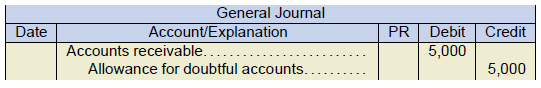
If Cambridge Instruments Co. pays $5,000 cash and indicates that this is all that the company can pay of the original $18,000, the entry would be:
Step 1: Reinstate the account receivable upon receipt of cash (reversing a portion of the write-off entry):
 Step 2: Record the receipt of cash on account from Cambridge Instruments:
Summary of Transactions and Adjusting Entries
An understanding of the relationships between the accounts receivable and the AFDA accounts and the types of transactions that affect them are important for sound accounts analysis. Below is an overview of some of the types of transactions that affect these accounts:
| Transaction of Adjusting Entry | Accounts Receivable | Allowance for Doubtful Accounts | ||
|---|---|---|---|---|
| Debit | Credit | Debit | Credit | |
| Opening balance, assuming accounts have normal balances | 1) $$ | 1) | $$ | |
| Sale on account | 2) $$ | 2) | ||
| Cash receipts | 3) | $$ | 3) | |
| Customer account written-off | 4) | $$ | 4) $$ | |
| Reinstatement of account previously written-off | 5) $$ | 5) | $$ | |
| End of period adjustment for uncollectible accounts (debit to bad debt expense) | 6) | 6) | $$ | |
| Closing balance, end of period | $$ | $$ | ||
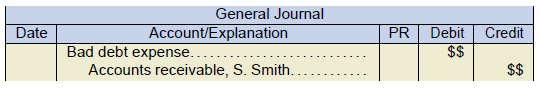
Direct Write-off of Uncollectible Accounts
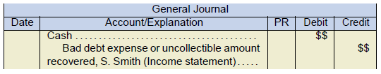
Some smaller companies may only have a few credit sales transactions and small ac- counts receivable balances. These companies usually use the simpler direct write-off method because the amount of uncollectible accounts is deemed to be immaterial. This means that when a specific customer account is determined to be uncollectible, the account receivable for that customer account is written-off with the debit entry recorded to bad debt expense as shown in the following entry:
If the uncollectible account written-off is subsequently collected at some later date, the entry would be:
If the uncollectible amounts were material, it would not be appropriate to use the direct write-off method, for many reasons:
- Without an estimate for uncollectible accounts, net account receivables would be reported at an amount higher than their net realizable value.
- The write-off of the uncollectible account will likely occur in a different year than the sale, which will create over- and under-statements of net income over the affected years resulting in non-compliance of the matching principle.
- Direct write-off creates an opportunity to manipulate asset amounts and net income. For example, management might delay a direct write-off to keep net income high artificially if this will favourably affect a bonus payment.
This section of the chapter is intended to be a summary overview of the methods and entries used to estimate and write-off uncollectible accounts originally covered in detail in the introductory accounting course. Students may wish to review those learning concepts from that course.
6.3.2. Notes Receivable
Recognition and Measurement of Notes Receivable
A note receivable is an unconditional written promise to pay a specific sum of money on demand or on a defined future date and is supported by a formal written promissory note. For this reason, notes are negotiable instruments the same as cheques and bank drafts.
Notes receivable can arise due to loans, advances to employees, or from higher-risk customers who need to extend the payment period of an outstanding account receivable. Notes can also be used for sales of property, plant, and equipment or for exchanges of long-term assets. Notes arising from loans usually identify collateral security in the form of assets of the borrower that the lender can seize if the note is not paid at the maturity date.
Notes may be referred to as interest-bearing or non-interest-bearing:
- Interest-bearing notes have a stated rate of interest that is payable in addition to the face value of the note.
- Notes with stated rates below the market rates or zero- or non-interest-bearing notes may or may not have a stated rate of interest. This is usually done to encourage sales. However, there is always an interest component embedded in the note, and that amount will be equal to the difference between the amount that was borrowed and the amount that will be repaid.
Notes may also be classified as short-term (current) assets or long-term assets on the balance sheet:
- Current assets: short-term notes that become due within the next twelve months (or within the business’s operating cycle if greater than twelve months);
- Long-term assets: notes are notes with due dates greater than one year.
Cash payments can be interest-only with the principal portion payable at the end or a mix of interest and principal throughout the term of the note.
Notes receivable are initially recognized at the fair value on the date that the note is legally executed (usually upon signing). Subsequent valuation is measured at amortized cost.
Transaction Costs
It is common for notes to incur transactions costs, especially if the note receivable is acquired using a broker, who will charge a commission for their services. For a company using either ASPE or IFRS, the transaction costs associated with financial assets such as notes receivable that are carried at amortized cost are to be capitalized which means that the costs are to be added to the asset’s fair value of the note at acquisition and subsequently included with any discount or premium and amortized over the term of the note.
Short-Term Notes Receivable
When notes receivable have terms of less than one year, accounting for short-term notes is relatively straightforward as discussed below.
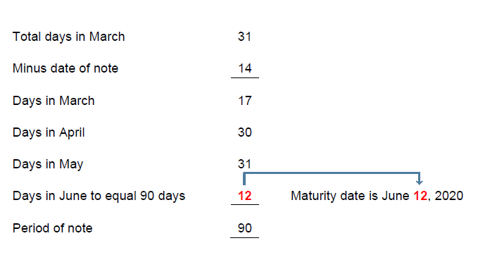
Calculating the Maturity Date
Knowing the correct maturity date will have an impact on when to record the entry for the note and how to calculate the correct interest amount throughout the note’s life. For example, to calculate the maturity date of a ninety-day note dated March 14, 2020:
Recall the formula for simple interest:
Interest = Principle × Rate × Time
For example, assume that on March 14, 2020, Ripple Stream Co. accepted a ninety- day, 8% note of $5,000 in exchange for extending the payment period of an outstanding account receivable of the same value. Ripple’s entry to record the acceptance of the note that will replace the accounts
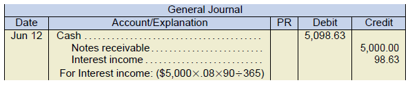
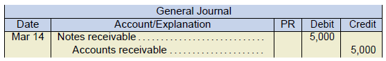 The entry for payment of the note ninety days at maturity on June 12 would be:
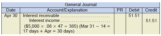
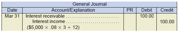
 In the example above, if financial statements are prepared during the time that the note receivable is outstanding, interest will be accrued to the reporting date of the balance sheet. For example, if Ripple’s year-end were April 30, the entry to accrue interest from March 14 to April 30 would be:
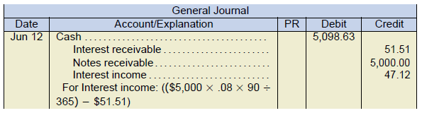
 When the cash payment occurs at maturity on June 12, the entry would be:
 The interest calculation will differ slightly had the note been stated in months instead of days. For example, assume that on January 1, Ripple Stream accepted a three-month (instead of a ninety-day), 8%, note in exchange for the outstanding accounts receivable. If Ripple’s year-end was March 31, the interest accrual would be:
Note the difference in the interest calculation between the ninety-day and the three-month notes recorded above. The interest amounts differ slightly between the two calculations because the ninety-day note uses a 90⁄365 ratio (or 24.6575% for a total amount of $98.63) while the three-month note uses a 3⁄12 ratio (or 25% for a total of $100.00).
Receivables, Interest, and the Time Value of Money
All financial assets are to be measured initially at their fair value which is calculated as the present value amount of future cash receipts. But what is present value? It is a discounted cash flow concept, which is explained next.
It is common knowledge that money deposited in a savings account will earn interest, or money borrowed from a bank will accrue interest payable to the bank. The present value of a note receivable is therefore the amount that you would need to deposit today, at a given rate of interest, which will result in a specified future amount at maturity. The cash flow is discounted to a lesser sum that eliminates the interest component—hence the term discounted cash flow. The future amount can be a single payment at the date of maturity or a series of payments over future time periods or some combination of both. Put into context for receivables, if a company must wait until a future date to receive the payment for its receivable, the receivable’s face value at maturity will not be an exact measure of its fair value on the date the note is legally executed because of the embedded interest component.
For example, assume that a company makes a sale on account for $5,000 and receives a $5,000, six-month note receivable in exchange. The face value of the note is therefore $5,000. If the market rate of interest is 9%, or its value without the interest component, is $4,780.79 and not $5,000. The $4,780.79 is the amount that if deposited today at an interest rate of 9% would equal $5,000 at the end of six months. Using an equation, the note can be expressed as:
(0 PMT, .75% I/Y, 6 N, 5000 FV)
- Where I/Y is interest of .75% each month (9% ÷ 12 months) for six months.
- N is for interest compounded each month for six months.
- FV is the payment at the end of six months’ time (future value) of $5,000.
To summarize, the discounted amount of $4,780.79 is the fair value of the $5,000 note at the time of the sale, and the additional amount received after the sale of $219.21 ($5,000.00 − $4,780.79) is interest income earned over the term of the note (six months). However, for any receivables due in less than one year, this interest income component is usually insignificant. For this reason, both IFRS and ASPE allow net realizable value (the net amount expected to be received in cash) to approximate the fair value for short- term notes receivables that mature within one year. So, in the example above, the $5,000 face value of the six-month note will be equivalent to the fair value and will be the amount reported, net of any estimated uncollectability (i.e. net realizable value), on the balance sheet until payment is received. However, for notes with maturity dates greater than one year, fair values are to be determined at their discounted cash flow or present value, which will be discussed next.
Long-Term Notes Receivable
The difference between a short-term note and a long-term note is the length of time to maturity. As the length of time to maturity of the note increases, the interest component becomes increasingly more significant. As a result, any notes receivable that are greater than one year to maturity are classified as long-term notes and require the use of present values to estimate their fair value at the time of issuance. After issuance, long-term notes receivable are measured at amortized cost. Determining present values requires an analysis of cash flows using interest rates and time lines, as illustrated next.
Present Values and Time Lines
The following timelines will illustrate how present value using discounted cash flows works. Below are three different scenarios:
- Assume that on January 1, Maxwell lends some money in exchange for a $5,000, five-year note, payable as a lump-sum at the end of five years. The market rate of interest is 5%. Maxwell’s year-end is December 31. The first step is to identify the amount(s) and timing of all the cash flows as illustrated below on the timeline. The amount of money that Maxwell would be willing to lend the borrower using the present value calculation of the cash flows would be $3,917.63 as follows:
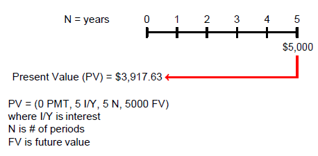 In this case, Maxwell will be willing to lend $3,917.63 today in exchange for a payment of $5,000 at the end of five years at an interest rate of 5% per annum. The entry for the note receivable at the date of issuance would be:
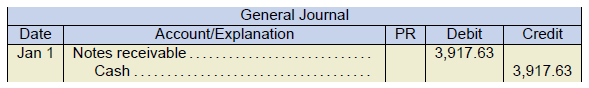
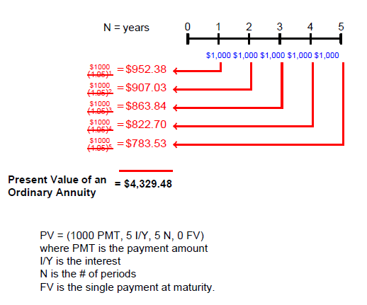
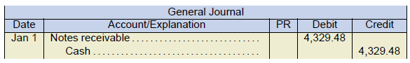
- Now assume that on January 1, Maxwell lends an amount of money in exchange for a $5,000, five-year note. The market rate of interest is 5%. The repayment of the note is payments of $1,000 at the end of each year for the next five years (present value of an ordinary annuity). The amount of money that Maxwell would be willing to lend the borrower using the present value calculation of the cash flows would be$4, 329.48 as follows:
 The entry for the note receivable would be:
Note that Maxwell is willing to lend more money ($4,329.48 compared to $3,917.63) to the borrower in this example. Another way of looking at it is that the interest component embedded in the note is less for this example. This makes sense because the principal amount of the note is being reduced over its five-year life because of the yearly payments of $1,000. - How would the amount of the loan and the entries above differ if Maxwell received five equal payments of $1,000 at the beginning of each year (present value of an annuity due) instead of at the end of each year as shown in scenario 2 above? The amount of money that Maxwell would be willing to lend using the present value calculation of the cash flows would be $4,545.95 as follows:
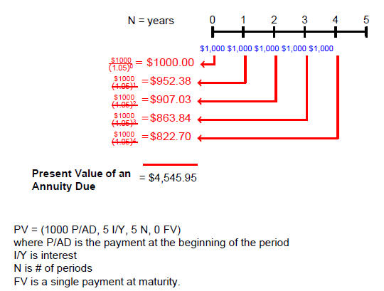 The entry for the note receivable would be:
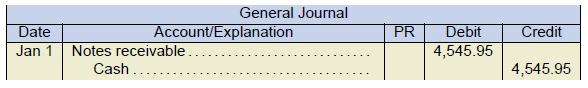
Again, the interest component will be less because a payment is paid immediately upon execution of the note, which causes the principal amount to be reduced sooner than a payment made at the end of each year.
Below is a comparison of the three scenarios:
|
Scenario 1 Single payment at maturity |
Scenario 2 Five payments of $1,000 at the end of each month |
Scenario 3 Five payments of $1,000 at the beginning of each month |
|
|---|---|---|---|
| Face value of the note | $5,000 | $5,000 | $5,000 |
| Less: present value of the note | 3,918 | 4,329 | 4,546 |
| Interest component | $1,082 | $671 | $454 |
Note that the interest component decreases for each of the scenarios even though the total cash repaid is $5,000 in each case. This is due to the timing of the cash flows as discussed earlier. In scenario 1, the principal is not reduced until maturity and interest would accrue over the full five years of the note. For scenario 2, the principal is being reduced on an annual basis, but the payment is not made until the end of each year. For scenario 3, there is an immediate reduction of principal due to the first payment of $1,000 upon issuance of the note. The remaining four payments are made at the beginning instead of at the end of each year. This results in a reduction in the principal amount owing upon which the interest is calculated.
This is the same concept as a mortgage owing for a house, where it is commonly stated by financial advisors that a mortgage payment split and paid every half-month instead of a single payment once per month will result in a significant reduction in interest costs over the term of the mortgage. The bottom line is: If there is less principal amount owing at any time over the life of a note, there will be less interest charged.
Present Values with Unknown Variables
As is the case with any algebraic equation, if all variables except one are known, the final unknown variable can be determined. For present value calculations, if any four of the five variables in equation PV = (PMT, I/Y, N, FV) are known, the fifth “unknown” variable amount can be determined using a business calculator or an Excel net present value function. For example, if the interest rate (I/Y) is not known, it can be derived if all the other variables in the equation are known. This will be illustrated when non-interest-bearing long-term notes receivable are discussed later in this chapter.
Present Values when Stated Interest Rates are Different than Effective (Market) Interest Rates
Differences between the stated interest rate (or face rate) and the effective (or market) rate at the time a note is issued can have accounting consequences as follows:
If the stated interest rate of the note (which is the interest rate that the note pays) is 10% at a time when the effective interest rate (also called the market rate, or yield) is 10% for notes with similar characteristics and risk, the note is initially recognized as:
face value = fair value = present value of the note
This makes intuitive sense since the stated rate of 10% is equal to the market rate of 10%.
If the stated interest rate is 10% and the market rate is 11%, the stated rate is lower than the market rate and the note is trading at a discount.
If stated rate lower than market ⇒ Present value lower ⇒ Difference is a discount
If the stated interest rate is 10% and the market rate is 9%, the stated rate is higher than the market rate and the note is trading at a premium.
If stated rate higher than market ⇒ Present value higher ⇒ Difference is a premium
The premium or discount amount is to be amortized over the term of the note. Below are the acceptable methods to amortize discounts or premiums:
- If a company follows IFRS, the effective interest method of amortization is required (discussed in the next section).
- If a company follows ASPE, the amortization method is not specified, so either straight-line amortization or the effective interest method is appropriate as an accounting policy choice.
Long-Term Notes, Subsequent Measurement
Under IFRS and ASPE, long-term notes receivable that are held for their cash flows of principal and interest are subsequently accounted for at amortized cost, which is calculated as:
- Amount recognized when initially acquired (present value) including any transaction costs such as commissions or fees
- Plus interest and minus any principal collections/receipts. Payments can also be blended interest and principal.
- Plus amortization of discount or minus amortization of premium
- Minus write-downs for impairment, if applicable
Below are some examples with journal entries involving various stated rates compared to market rates.
1. Notes Issued at Face Value
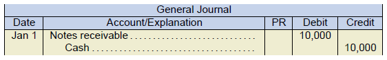
Assume that on January 1, Carpe Diem Ltd. lends $10,000 to Fascination Co. in exchange for a $10,000, three-year note bearing interest at 10% payable annually at the end of each year (ordinary annuity). The market rate of interest for a note of similar risk is also 10%. The note’s present value is calculated as:
| Face value of the note | $10,000 |
|---|---|
| Present value of the note principle and interest:
Interest = $10,000 × 10% = $1,000PMT PV = (1000 PMT, 10 I/Y, 3N, 10000FV) |
10,000 |
| Difference | $0 |
In this case, the note’s face value and present value (fair value) are the same ($10,000) because the effective (market) and stated interest rates are the same. Carpe Diem’s entry on the date of issuance is:
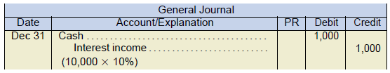
If Carpe Diem’s year-end was December 31, the interest income recognized each year would be:
2. Stated Rate Lower than Market Rate: A Discount
Assume that Anchor Ltd. makes a loan to Sizzle Corp. in exchange for a $10,000, three- year note bearing interest at 10% payable annually. The market rate of interest for a note of similar risk is 12%. Recall that the stated rate of 10% determines the amount of the cash received for interest; however, the present value uses the effective (market) rate to discount all cash flows to determine the amount to record as the note’s value at the time of issuance. The note’s present value is calculated as:
| Face value of the note | $10,000 |
|---|---|
| Present value of the note principal and interest:
Interest = $10,000 × 10% = $1,000 PMT PV = (1000 PMT, 12 I/Y, 3 N, 10000 FV) |
9,520 |
| Difference | $480 |
As shown above, the note’s market rate (12%) is higher than the stated rate (10%), so the note is issued at a discount.
Anchor’s entry to record the issuance of the note receivable:
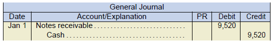
Even though the face value of the note is $10,000, the amount of money lent to Sizzle would only be $9,520, which is net of the discount amount and is the difference between the stated and market interest rates discussed earlier. In return, Anchor will receive an annual cash payment of $1,000 for three years plus a lump sum payment of $10,000 at the end of the third year, when the note matures. The total cash payments received will be $13,000 over the term of the note, and the interest component of the note would be:
Cash received
Present value (fair value)
Interest income component
$13,000
9,520
3,480 (over the three-year life)
As mentioned earlier, if Anchor used IFRS the $480 discount amount would be amortized using the effective interest method. If Anchor used ASPE, there would be a choice between the effective interest method and the straight-line method.
Below is a schedule that calculates the cash received, interest income, discount amortization, and the carrying amount (book value) of the note at the end of each year using the effective interest method:
|
$10,000 Note Receivable Payment and Amortization Schedule |
||||
|---|---|---|---|---|
| Cash Received | Interest Income @ 12% | Amortized Discount | Carrying Amount | |
| Date of issue | $9,520 | |||
| End of Year 1 | $1,000 | $1,142[1] | $142 | 9,662 |
| End of Year 2 | 1,000 | 1,159 | 159 | 9,821 |
| End of year 3 | 1,000 | 1,179 | 179 | 10,000 |
| End of year 3 final payment | 10,000 | – | – | 0 |
| $13,000 | $3,480 | $480 | ||
The total discount $480 amortized in the schedule is equal to the difference between the face value of the note of $10,000 and the present value of the note principal and interest of $9,250. The amortized discount is added to the note’s carrying value each year, thereby increasing its carrying amount until it reaches its maturity value of $10,000. As a result, the carrying amount at the end of each period is always equal to the present value of the note’s remaining cash flows discounted at the 12% market rate. This is consistent with the accounting standards for the subsequent measurement of long-term notes receivable at amortized cost.
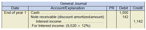
If Anchor’s year-end was the same date as the note’s interest collected, at the end of year 1 using the schedule above, Anchor’s entry would be:
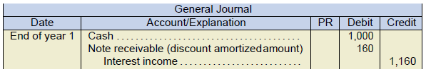
Alternatively, if Anchor used ASPE the straight-line method of amortizing the discount is simple to apply. The total discount of $480 is amortized over the three-year term of the note in equal amounts. The annual amortization of the discount is $160 ($480 ÷ 3 years) for each of the three years as shown in the following entry:
Comparing the three years’ entries for both the effective interest and straight-line methods shows the following pattern for the discount amortization of the note receivable:
| Effective Interest | Straight-Line | |
|---|---|---|
| End of year 1 | $142 | $160 |
| End of year 2 | 159 | 160 |
| End of year 3 | 179 | 160 |
| $480 | $480 |
The amortization of the discount using the effective interest method results in increasing amounts of interest income that will be recorded in the adjusting entry (decreasing amounts of interest income for amortizing a premium) compared to the equal amounts of interest income using the straight-line method. The straight-line method is easier to apply but its shortcoming is that the interest rate (yield) for the note is not held constant at the 12% market rate as is the case when the effective interest method is used. This
is because the amortization of the discount is in equal amounts and does not take into consideration what the carrying amount of the note was at any given period of time. At the end of year 3, the notes receivable balance is $10,000 for both methods, so the same entry is recorded for the receipt of the cash.
3. Stated Rate More than Market Rate: A Premium
Had the note’s stated rate of 10% been greater than a market rate of 9%, the present value would be greater than the face value of the note due to the premium. The same types of calculations and entries as shown in the previous illustration regarding a discount would be used. Note that the premium amortized each year would decrease the carrying amount of the note at the end of each year until it reaches its face value amount of $10,000.
|
$10,000 Note Receivable Payment and Amortization Schedule |
||||
|---|---|---|---|---|
| Cash Received | Interest Income @ 9% | Amortized Premium | Carrying Amount | |
| Date of issue | $10,253 | |||
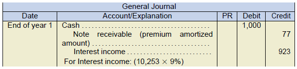
| End of year 1 | $1,000 | $923[2] | $77 | 10,176 |
| End of year 2 | 1,000 | 916 | 84 | 10,091 |
| End of year 3 | 1,000 | 908 | 92 | 10,000 |
| End of year 3 final payment | 10,000 | – | – | 0 |
| $13,000 | $2,727 | $253 | ||
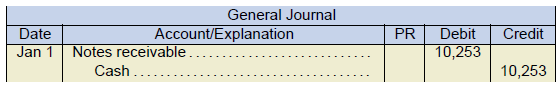
Anchor’s entry on the note’s issuance date is for the present value amount (fair value):
If the company’s year-end was the same date as the note’s interest collected, at the end of year 1 using the schedule above, the entry would be:
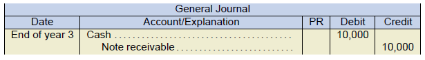
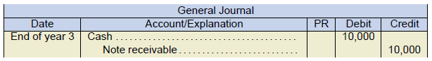
 The entry when paid at maturity would be:
4. Zero-Interest Bearing Notes
Some companies will issue zero-interest-bearing notes as a sales incentive. The notes do not state an interest rate but the term “zero-interest” is inaccurate because financial instruments always include an interest component that is equal to the difference between the cash lent and the higher amount of cash repaid at maturity. Even though the interest rate is not stated, the implied interest rate can be derived because the cash values lent and received are both known. In most cases, the transaction between the issuer and acquirer of the note is at arm’s length, so the implicit interest rate would be a reasonable estimate of the market rate.
Assume that on January 1, Eclipse Corp. received a five-year, $10,000 zero-interest bearing note. The amount of cash lent to the issuer (which is equal to the present value) is $7,835 (rounded). Eclipse’s year-end is December 31. Looking at the cash flows and the time line:
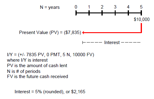
Notice that the sign for the $7,835 PV is preceded by the ± symbol, meaning that the PV amount is to have the opposite symbol to the $10,000 FV amount, shown as a positive value. This is because the FV is the cash received at maturity or cash inflow (positive value), while the PV is the cash lent or a cash outflow (opposite or negative value). Many business calculators require the use of a ± sign for one value and no sign (or a positive value) for the other to calculate imputed interest rates correctly. Consult your calculator manual for further instructions regarding zero-interest note calculations.
The implied interest rate is calculated to be 5% and the note’s interest component (rounded) is $2,165 ($10,000 − $7,835), which is the difference between the cash lent and the higher amount of cash repaid at maturity. Below is the schedule for the interest and amortization calculations using the effective interest method.
| Non-Interest-Bering Note Receivable Payment and Amortization Schedule Effective Interest Method | ||||
|---|---|---|---|---|
| Cash Received | Interest Income @5% | Amortized Discount | Carrying Amount | |
| Date of issue | $7,835,26 | |||
| End of year 1 | $0 | $391.76[3] | $391.76 | 8,227.02 |
| End of year 2 | 0 | 411.35 | 411.35 | 8,638.37 |
| End of year 3 | 0 | 431.92 | 431.92 | 9,070.29 |
| End of year 4 | 0 | 453.51 | 453.51 | 9,523.81 |
| End of year 5 | 0 | 476.19 | 475.19 | 10,000.00 |
| End of year 5 payment | 10,000 | 0 | ||
| $2,164.74 | $2,164.74 | |||
Remember – for zero-interest notes, you can re-arrange the present value formula to calculate the interest rate if needed.
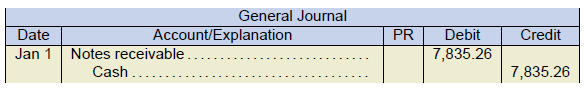
The entry for the note receivable when issued would be:
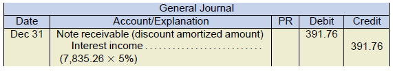
At Eclipse’s year-end of December 31, the interest income at the end of the first year using the effective interest method would be:
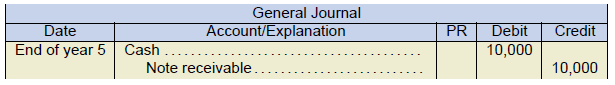
At maturity when the cash interest is received, the entry would be:
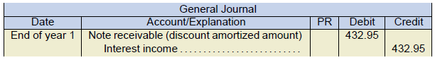
If Eclipse used ASPE instead of IFRS, the entry using straight-line method for amortizing the discount is calculated as the total discount of $2,164.74, amortized over the five-year term of the note resulting in equal amounts each year. Therefore, the annual amortization is $432.95 ($2,164.74 ÷ 5 years) each year is recorded as:
5. Notes Receivable in Exchange for Property, Goods, or Services
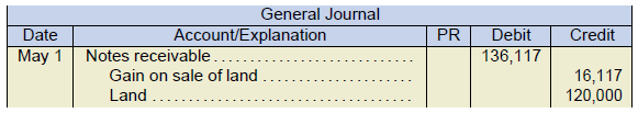
When property, goods, or services are exchanged for a note, and the market rate and the timing and amounts of cash received are all known, the present value of the note can be determined. For example, assume that on May 1, Hudson Inc. receives a $200,000, five-year note in exchange for land originally costing $120,000. The market rate for a note with similar characteristics and risks is 8%. The present value is calculated as follows:
PV = (0 PMT, 8 I/Y, 5 N, 200000 FV)
PV = $136,117
The entry upon issuance of the note and sale of the land would be:
However, if the market rate is not known, either of following two approaches can be used to determine the fair value of the note:
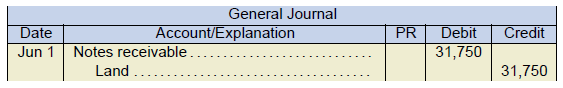
- Determine the fair value of the property, goods, or services given up. As was discussed for zero-interest bearing notes where the interest rate was not known, the implicit interest rate can still be derived because the cash amount lent, and the timing and amount of the cash flows received from the issuer are both known. In this case the amount lent is the fair value of the property, goods, or services given up. Once the interest is calculated, the effective interest method can be applied.[4]For example, on June 1, Mayflower Consulting Ltd. receives a $40,000, three-year note in exchange for some land. The market rate cannot be accurately determined due to credit risks regarding the issuer. The land cost and fair value is $31,750. The interest rate is calculated as follows:I/Y = (±31750 PV, 0 PMT, 3 N, 40000 FV)I/Y = 8%; the interest income component is $8,250 over three years ($40,000 − $31,750)The entry upon issuance of the note would be:
-
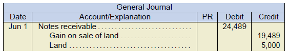
Determine an imputed interest rate. An imputed interest rate is an estimated interest rate used for a note with comparable terms, conditions, and risks between an independent borrower and lender. On June 1, Edmunds Co. receives a $30,000, three-year note in exchange for some swampland. The land has a historic cost of $5,000 but neither the market rate nor the fair value of the land can be determined. In this case, a market rate must be imputed and used to determine the note’s present value. The rate will be estimated based on interest rates currently in effect for companies with similar characteristics and credit risk as the company issuing the note. For IFRS companies, the “evaluation hierarchy” identified in IFRS 13 Fair Value Measurement would be used to determine the fair value of the land and the imputed interest rate. In this case, the imputed rate is determined to be 7%. The present value is calculated as follows:
PV = (7 I/Y, 3 N, 30000 FV)PV = $24,489)
The entry upon issuance of the note would be:
It’s important to note. Whether we are selling a good or service OR is a short-term accounts receivable becomes a long-term note receivable, the accounting is very similar.
Loans to employees
In cases where there are non-interest-bearing long-term loans to company employees, the fair value is determined by using the market rate for loans with similar characteristics, and the present value is calculated on that basis. The amount loaned to the employee invariably will be higher than the present value using the market rate because the loan is intended as a reward or incentive. This difference would be deemed as additional compensation and recorded as Compensation expense.
Impairment of notes receivable
Just as was the case with accounts receivable, there is a possibility that the holder of the note receivable will not be able to collect some or all of the amounts owing. If this happens, the receivable is considered impaired. When the investment in a note receivable becomes impaired for any reason, the receivable is re-measured at the present value of the currently expected cash flows at the loan’s original effective interest rate.
The impairment amount is recorded as a debit to bad debt expense and as a credit either to an allowance for uncollectible notes account (a contra account to notes receivable) or directly as a reduction to the asset account.
6.3.3. Derecognition and Sale of Receivables: Shortening the Credit-to-Cash Cycle
Derecognition is the removal of a previously recognized receivable from the company’s balance sheet. In the normal course of business, receivables arise from credit sales and, once paid, are removed (derecognized) from the books. However, this takes valuable time and resources to turn receivables into cash. As someone once said, “turnover is vanity, profit is sanity, but cash is king”[5]. Simply put, a business can report all the profits possible, but profits do not mean cash resources. Sound cash flow management has always been important but, since the economic downturn in 2008, it has become the key to survival for many struggling businesses. As a result, companies are always looking for ways to shorten the credit-to-cash cycle to maximize their cash resources. Two such ways are secured borrowings and sales of receivables, discussed next.
Secured Borrowings
Companies often use receivables as collateral for a loan or a bank line of credit. The receivables are pledged as security for the loan, but the control and collection often remain with the company, so the receivables are left on the company’s books. The company records the proceeds of the loan received from the finance company as a liability with the loan interest and any other finance charges recorded as expenses. If a company defaults on its loan, the finance company can seize the secured receivables and directly collect the cash from the receivables as payment against the defaulted loan. This will be illustrated in the section on factoring, below.
Sales of Receivables
What is the accounting treatment if a company’s receivables are transferred (sold) to a third party (factor)? Certain industry sectors, such as auto dealerships and almost all small- and medium-sized businesses selling high-cost goods (e.g., gym equipment retailers) make extensive use of third-party financing arrangements with their customers to speed up the credit-to-cash cycle. Whether a receivable is transferred to a factor (sale) or held as security for a loan (borrowing) depends on the criteria set out in IFRS and ASPE which are discussed next.
Conditions for Treatment as a Sale
For accounting purposes, the receivables should be derecognized as a sale when they meet the following criteria:
IFRS – substantially all of the risks and rewards have been transferred to the factor.
The evidence for this is that the contractual rights to receive the cash flows have been transferred (or the company continues to collect and forward all the cash it collects without delay) to the factor. As well, the company cannot sell or pledge any of these receivables to any third parties other than to the factor.
ASPE – control of the receivables has been surrendered by the transferor. This is evidenced when the following three conditions are all met:
- The transferred assets have been isolated from the transferor.
- The factor has obtained the right to pledge or to sell the transferred assets.
- The transferor does not maintain effective control of the transferred assets through a repurchase agreement.
If the conditions for either IFRS or ASPE are not met, the receivables remain in the accounts and the transaction is treated as a secured borrowing (recorded as a liability) with the receivables as security for the loan. The accounting treatment regarding the sale of receivables using either standard is a complex topic; the discussion in this section is intended as a basic overview.
Below are some different examples of sales of receivables; such as factoring and securitization.
Factoring
Factoring is when individual accounts receivable are sold or transferred to a recipient or factor, usually a financial institution, in exchange for cash minus a fee called a discount. The seller does not usually have any subsequent involvement with the receivable and the factor collects directly from the customer. (Companies selling fitness equipment exclusively use this method for all their credit sales to customers.)
The downside to this strategy is that factoring is expensive. Factors typically charge a 2% to 3% fee when they buy the right to collect payments from customers. A 2% discount for an invoice due in thirty days is the equivalent of a substantial 25% a year, and 3% is over 36% per year compared to the much lower interest rates charged by banks and finance companies. Most companies are better off borrowing from their bank, if it is possible to do so.
However, factors will often advance funds when more traditional banks will not. Even with only a prospective order in hand from a customer, a business can turn to a factor to see if it will assume or share the risk of the receivable. Without the factoring arrangement, the business must take time to secure and collect the receivable; the factor offers a reduction in additional effort and aggravation that may be worth the price of the fee paid to the factor.
There are risks associated with factoring receivables. Companies that intend to sell their receivables to a factor need to check out the bank and customer references of any factor. There have been cases where a factor has gone out of business, still owing the company substantial amounts of money held back in reserve from receivables already paid up.
Factoring Versus Borrowing: A Comparison
The difference between factoring and borrowing can be significant for a company that wants to sell some or all of its receivables. Consider the following example:
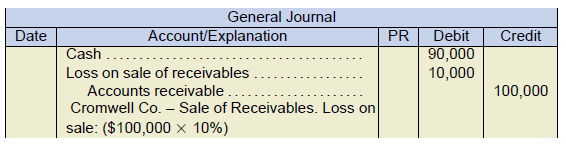
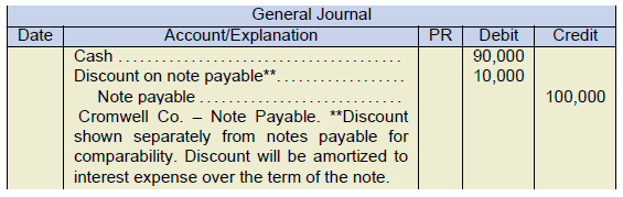
Assume that on June 1, Cromwell Co. has $100,000 accounts receivable it wants to sell to a factor that charges 10% as a financing fee. Below is the transaction recorded as a sale of receivables compared to a secured note payable arrangement, starting with some opening balances:
| Cromwell Co. Balance Sheet – Opening Balances | |
|---|---|
| Cash | $10,000 |
| Accounts receivable | 150,000 |
| Property, plant, and equipment | 200,000 |
| Total assets | $360,000 |
| Accounts payable | $70,000 |
| Note payable | 0 |
| Equity | 290,000 |
| Total liabilities and equity | $360,000 |
| Debt-to-total assets ratio | 19% |
The journal entry to record the sale of the receivables (factoring):
 Below is the balance sheet after the transaction:
| Cromwell Co. Balance Sheet – Sale of Receivables | |
|---|---|
| Cash | $100,000 |
| Accounts receivable | 50,000 |
| Property, plant, and equipment | 200,000 |
| Total assets | $350,000 |
| Accounts payable | $70,000 |
| Note payable | 0 |
| Equity | 280,000 |
| Total liabilities and equity | $350,000 |
| Debt-to-total assets ratio | 20% |
| Cromwell Co. Balance Sheet – Note Payable | |
|---|---|
| Cash | $100,000 |
| Accounts receivable | 150,000 |
| Property, plant, and equipment | 200,000 |
| Total assets | $450,000 |
| Accounts payable | $70,000 |
| Note payable | 90,000 |
| Equity | 290,000 |
| Total liabilities and equity | $450,000 |
| Debt-to-total assets ratio | 36% |
Note that the entry for a sale is straightforward with the receivables of $100,000 derecognized from the accounts and a decrease in retained earnings due to the loss reported in net income. However, for a secured borrowing, a note payable of $90,000 is added to the accounts as a liability, and the accounts receivable of $100,000 remains in the accounts as security for the note payable. Referring to the journal entry above, in both cases cash flow increased by $90,000, but for the secured borrowing, there is added debt of $90,000, affecting Cromwell’s debt ratio and negatively impacting any restrictive covenants Cromwell might have with other creditors. After the transaction, the debt-to- total assets ratio for Cromwell is 20% if the accounts receivable transaction meets the criteria for a sale. The debt ratio worsens to 36% if the transaction does not meet the criteria for a sale and is treated as a secured borrowing. This impact could motivate managers to choose a sale for their receivables to shorten the credit-to-cash cycle, rather than the borrowing alternative.
Sales without Recourse
If receivables are sold without recourse, the purchasers assumes the risk of collection and is responsible for any credit losses. This type of a transfer is considered to be an outright sale of the receivables.
For sales without recourse, all the risks and rewards (IFRS) as well as the control (ASPE) have been transferred to the factor, and the selling company no longer has any involvement.
For example, assume that on August 1, Ashton Industries Ltd. factors $200,000 of accounts receivable with Savoy Trust Co., the factor, on a without-recourse basis. All the risks, rewards, and control are transferred to the finance company, which charges an 8% fee and withholds a further 4% of the accounts receivables for estimated returns and allowances. The entry for Ashton is:
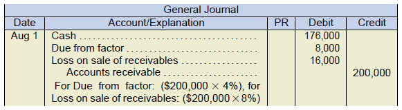
The accounting treatment will be the same for IFRS and ASPE since both sets of con- ditions (risks and rewards and control) have been met. If no returns and allowances are given to customers owing the receivables, Ashton will recoup the $8,000 from the factor. In turn, Savoy’s net income will be the $16,000 revenue reduced by any uncollectible receivables, since it now has assumed the risks/rewards and control of these receivables.
Sales with Recourse
If receivables are sold with recourse, the seller guarantees payment to the purchaser of the receivables, if the customer fails to pay.
In this case, Ashton guarantees payment to Savoy for any uncollectible receivables (re- course obligation). Under IFRS, the guarantee means that the risks and rewards have not been transferred to the factor, and the accounting treatment would be as a secured borrowing as illustrated above in Cromwell—Note Payable. Under ASPE, if all three conditions for treatment as a sale as described previously are met, the transaction can be treated as a sale.
Continuing with the example for Ashton, assume that the receivables are sold with re- course, the company uses ASPE, and that all three conditions have been met. In addition to the 8% fee and 4% withholding allowance, Savoy estimates that the recourse obligation has a fair value of $5,000. The entry for Ashton, including the estimated recourse obligation is:
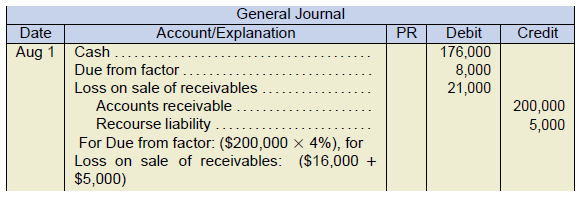 You will see that the recourse liability to Savoy results in an increase in the loss on sale of receivables by the recourse liability amount of $5,000. If there were no uncollectible receivables, Ashton will eliminate the recourse liability amount and decrease the loss. Savoy’s net income will be the finance fee of $16,000 with no reductions in revenue due to uncollectible accounts, since these are being guaranteed and assumed by Ashton.
Securitization
Securitization is a financing transaction that gives companies an alternative way to raise funds other than by issuing debt, such as a corporate bond or note. The process is extremely complex and the description below is a simplified version.
The receivables are sold to a holding company called a Special Purpose Entity (SPE), which is sponsored by a financial intermediary. This is similar to factoring without re- course, but is done on a much larger scale. This sale of receivables and their removal from the accounting records by the company holding the receivables is an example of off- balance sheet accounting. In its most basic form, the securitization process involves two steps:
Step 1: A company (the asset originator) with receivables (e.g., auto loans, credit card debt), identifies the receivables (assets) it wants to sell and remove from its balance sheet. The company divides these into bundles, called tranches, each containing a group of receivables with similar credit risks. Some bundles will contain the lowest risk receivables (senior tranches) while other bundles will have the highest risk receivables (junior tranches).
The company sells this portfolio of receivable bundles to a special purpose entity (SPE) that was created by a financial intermediary specifically to purchase these types of portfolio assets. Once purchased, the originating company (seller) derecognizes the receivables and the SPE accounts for the portfolio assets in its own accounting records. In many cases, the company that originally sold the portfolio of receivables to the SPE continues to service the receivables in the portfolio, collects payments from the original borrowers and passes them on—less a servicing fee—directly to the SPE. In other cases, the originating company is no longer involved and the SPE engages a bank or financial intermediary to collect the receivables as a collecting agent.
Step 2: The SPE (issuing agent) finances the purchase of the receivables portfolio from the originating company by issuing tradeable interest-bearing securities that are secured or backed by the receivables portfolio it now holds in its own accounting records as stated in Step 1—hence the name asset-backed securities (ABS). These interest-bearing ABS securities are sold to capital market investors who receive fixed or floating rate payments from the SPE, funded by the cash flows generated by the portfolio collections. To summarize, securitization represents an alternative and diversified source of financing based on the transfer of credit risk (and possibly also interest rate and currency risk) from the originating company and ultimately to the capital market investors.
The Downside of Securitization
Securitization is inherently complex, yet it has grown exponentially. The resulting highly competitive securitization markets with multiple securitizers (financial institutions and SPEs), increase the risk that underwriting standards for the asset-backed securities could decline and cause sharp drops in the bundled or tranched securities’ market values. This is because both the investment return (principal and interest repayment) and losses are allocated among the various bundles according to their level of risk. The least risky bundles, for example, have first call on the income generated by the underlying receivables assets, while the riskiest bundles have last claim on that income, but receive the highest return.
Typically, investors with securities linked to the lowest-risk bundles would have little expectation of portfolio losses. However, because investors often finance their investment purchase by borrowing, they are very sensitive to changes in underlying receivables assets’ quality. This sensitivity was the initial source of the problems experienced in the sub-prime mortgage market (derivatives) meltdown in 2008. At that time, repayment issues surfaced in the riskiest bundles due to the weakened underwriting standards, and lack of confidence spread to investors holding even the lowest risk bundles, which caused panic among investors and a flight into safer assets, resulting in a fire sale of securitized debt of the SPEs.
In the future, securitized products are likely to become simpler. After years of posting virtually no capital reserves against high-risk securitized debt, SPEs will soon be faced with regulatory changes that will require higher capital charges and more comprehensive valuations. Reviving securitization transactions and restoring investor confidence might also require SPEs to retain an interest in the performance of securitized assets at each level of risk (Jobst, 2008).
6.3.4. Disclosures of Receivables
The standards for receivables reporting and disclosures have been in a constant state of change. IFRS 7 (IFRS, 2015) and IAS 1 (IAS, 2003) include significant disclosure requirements that provide information based on significance and the nature and extent of risks.
The Significance of Financial Instruments
IFRS 7 and IAS 1 specify the separate reporting categories based on significance such as the following:
- Trade accounts, amounts owing from related parties, prepayments, tax refunds, and other significant amounts
- Current amounts from non-current amounts
- Any impaired balances and amount of any allowance for credit risk and a reconciliation of the changes in the allowance account during the accounting period
- Disclosure on the income statement of the amounts of interest income, impairment losses, and any reversals associated with impairment losses
- Net losses on sales of receivables (IFRS, 2015, 7.20 a, iv).
For each receivables category above, the following disclosures are required:
- The carrying amounts such as amortized cost/cost and fair values (including meth- ods used to estimate fair value) with details of any amounts reclassified from one category to another or changes in fair values
- Carrying amount and terms and conditions regarding financial assets pledged as collateral or any financial assets held as collateral
- An indication of the amounts and, where practicable, the maturity dates of accounts with a maturity of more than one year
- For IFRS, extensive disclosures of major terms regarding the securitization or transfers of receivables, whether these have been derecognized in their entirety or not. Some of these disclosures include the characteristics of the securitization, the fair value measurements and methods used and cash flows, as well as the nature of the servicing requirements and associated risks.
The Nature and Extent of Risks Arising from Financial Instruments
Stakeholders, such as investors and creditors, want to know about the various transactions that hold risks. Basic types of risks and related disclosures are:
- Credit risk—the risk that one party to a financial instrument will default on its debt obligation. Disclosures include an analysis of the age of financial assets that are past due as at the end of the reporting period but not impaired and an analysis of financial assets that are individually determined to be impaired as at the end of the reporting period, including the factors the entity considered in determining that they are impaired (IFRS, 2015, 7.37 a, b).
- Liquidity risk—the risk that an entity will have difficulties in paying its financial liabilities.
- Market risk—the risk that the fair value or cash flows of a receivable will fluctuate due to changes in market prices which are affected by interest rate risk, currency risk, and other price risks. Disclosures include a sensitivity analysis for each type of market risk to which the entity is exposed at the end of the reporting period, showing how profit or loss and equity would have been affected by changes in the relevant risk variable that were reasonably possible at that date (IFRS, 2015, 7.40 a).
In addition, information about company policies for managing risk, including quantitative and qualitative data, is to be disclosed. ASPE disclosure requirements are much the same as IFRS, though perhaps requiring slightly less information about risk exposures and fair values than IFRS (CPA Canada, 2016, Part II, Section 3856.38–42).
- $9,520 × 12% = $1,142 ↵
- $10,253 × 9% = $923 ↵
- $7,845.26 × 5% = $391.76 ↵
- Source: http://www.iasplus.com/en/standards/ifrs/ifrs13 IFRS 13 Fair Value Measurement applies to IFRSes that require or permit fair value measurements or disclosures and provides a single IFRS framework for measuring fair value and requires disclosures about fair value measurement. The Standard defines fair value on the basis of an “exit price” notion and uses a “fair value hierarchy,” which results in a market-based, rather than entity-specific, measurement. IFRS 13 was originally issued in May 2011 and applies to annual periods beginning on or after 1 January 2013 and is beyond the scope of this course. For simplicity, the fair value of the property, goods or services given up as explained in the chapter material assumes that IFRS 13 assumptions and hierarchy to determine fair values have been appropriately considered. ↵
- “Cash is king” is a catch phrase for “cash is most important.” While a firm can generate a profit, if it cannot be converted to cash fast enough to pay the liabilities as they are due, then the company runs the risk of failing. ↵
