10.2 Depreciation Calculations
10.2.1. Depreciable Amount
The first element that needs to be determined for a depreciation calculation is the depreciable amount. It represents the cost that will be allocated to future periods through the depreciation process. This amount is determined by taking the asset’s cost and deducting the residual value. (Note: if the company uses the revaluation method, the cost is replaced by the revalued amount in this calculation.) The residual value is the estimated net amount that the company would be able to sell the asset for at the end of its useful life, based on current conditions. Thus, the estimate does not try to anticipate future changes in market or economic conditions; it merely considers the nature of the asset itself. The residual value is, of course, an estimate and is thus subject to possible error. As a result, IFRS requires an annual review of residual amounts used in depreciation calculations. If the residual amount needs to be changed, it should be accounted for prospectively as a change in estimate. Many assets will have a residual value of zero or close to zero, and this amount will thus be ignored in the calculation. If the revised residual value were to exceed the carrying value of the asset, then depreciation would cease until the residual value dropped back below the carrying value.
10.2.2. Useful Life
The useful life of an asset is determined by its utility to the company. This means that estimates need to be made about how long the company plans to use the asset. For certain types of assets, companies may have a policy of timed replacement, even if the asset is still functioning. This means the useful life may be less than the physical life of the asset. IFRS (International Accounting Standards, n.d., 16.56) identifies the following factors that need to be considered in determining useful life to the company:
- The expected usage of the asset, as assessed by reference to the asset’s expected capacity or physical output.
- The expected physical wear and tear, which depends on operational factors, such as the number of shifts for which the asset is to be used, the repair and maintenance program, and the care and maintenance of the asset while idle.
- The technical or commercial obsolescence of the asset arising from changes or improvements in production or from a change in the market demand for the product or service output of the asset. Expected future reductions in the selling price of an item that was produced using an asset could indicate the expectation of technical or commercial obsolescence of the asset, which, in turn, might reflect a reduction of the future economic benefits embodied in the asset.
- The legal or similar limits on the use of the asset, such as the expiry dates of related leases.
It should be apparent that a substantial amount of judgment is required in determining the useful life of an asset. Although management may have significant experience in working with these assets, the estimation process can still result in errors. The process of annual review and estimation changes for useful lives is the same as described above, in 10.2.1: Depreciable Amount, for residual values.
Another question that needs to addressed when determining the useful life of an asset is when to start and stop depreciating it. Depreciation of the asset should commence when the asset is available for use. This means that the asset is in place and ready for productive function, even if it is not actually being used yet. Depreciation should stop at the earlier date when the asset is either reclassified as held for sale or derecognized. These situations will be covered later in the chapter.
10.2.3. Methods of Calculation
The IFRS requirement of allocation of cost on a systematic basis is a deliberately vague description of the techniques used to calculate depreciation. Companies are given the freedom to choose the method used, as long as the method makes sense in relation to the consumption of future economic benefits realized by use of the asset. The standard does identify three broad techniques that can be used: straight line, diminishing balance, and units of production. However, other techniques could be justified if they provide a more systematic and reasonable allocation of cost. The standard also indicates that depreciation methods based on revenue should not be used, as revenue may be affected by factors, such as inflation, that are not directly related to the consumption of economic benefits.
The three main methods of calculating depreciation are:
- Straight-line method – is considered a function of the passage of time. Depreciation expense is usually the same every period (except at acquisition and disposal).
- Diminishing balance method – a type of decreasing charge or accelerated method which creates higher depreciation expense in the earlier years and lower depreciation expense in later periods.
- Activity method – is a variable-charge approach where depreciation expense will depend on the activity related to the asset.
Straight-Line Method
This is the simplest and most commonly used depreciation method. This method simply allocates cost in equal proportions to the time periods of an asset’s useful life. The formula to determine the depreciation charge is as follows:
For example, consider an automated packaging machine purchased for $100,000 that is used in a factory. It is estimated that this machine will have a useful life of ten years and will have a residual value of $5,000. The calculation of the annual depreciation charge is as follows:
The benefit of this method is its simplicity for both the preparer and reader of the financial statement. No special knowledge is required to understand the logic of the calculation. As well, the method is appropriate if we assume that economic benefits are delivered in roughly equal proportions over the life of the asset. However, there are arguments that are contrary to this assumption. For certain assets, it may be reasonable to assume that the economic benefits decline with the age of the asset, as there is more downtime due to repairs or other operational inefficiencies that result from age. If these inefficiencies are significant, then the straight-line method may not be the most appropriate method.
Diminishing-Balance Method
The diminishing-balance method results in more depreciation in the early years of an asset’s life and less depreciation in later years. The justification for this method is that an asset will offer its greatest service potential when it is relatively new. Once an asset ages and starts to require more repairs, it will be less productive to the business. This reasoning is quite consistent with the experience many companies have with assets that have mechanical components. This method will also result in an overall expense to the company that is fairly consistent over the life of the asset. In early years, depreciation charges are high, but repairs are low; in later years, this situation will reverse.
A number of different calculations can be used when applying the diminishing-balance method. The common feature of all the methods is that a constant percentage is applied to the closing net book value of the asset each year to determine the depreciation charge. The percentage that is used can be derived in a number of ways. The most accurate way would be to apply a formula to determine the exact percentage needed to depreciate the asset down to its residual value. Although this can be done, this approach is not often used, because it requires a more complex calculation. A simpler, more commonly used approach is to simply use a multiple based on the asset’s useful life. For example, a technique referred to as double-declining balance would convert the useful life to a percentage and multiply the result by two. In our previous example, the calculation would be as follows:
(1 ÷ Useful life) × 2 = Depreciation rate
(1 ÷ 10 years) × 2 = 20%
Depreciation would thus be calculated as follows:
| Year | Book Value, Opening | Rate | Depreciation Expense | Accumulated Depreciation | Book Value, Closing |
|---|---|---|---|---|---|
| 1 | 100,000 | 20% | 20,000 | 20,000 | 80,000 |
| 2 | 80,000 | 20% | 16,000 | 36,000 | 64,000 |
| 3 | 64,000 | 20% | 12,800 | 48,800 | 51,200 |
| 4 | 51,200 | 20% | 10,240 | 59,040 | 40,960 |
| 5 | 40,960 | 20% | 8,192 | 67,232 | 32,768 |
| 6 | 32,768 | 20% | 6,554 | 73,786 | 26,214 |
| 7 | 26,214 | 20% | 5,243 | 79,029 | 20,971 |
| 8 | 20,971 | 20% | 4,194 | 83,223 | 16,777 |
| 9 | 16,777 | 20% | 3,355 | 86,578 | 13,422 |
| 10 | 13,422 | 20% | 8,422[1] | 95,000 | 5,000 |
Also note that in the calculations above, unlike other methods, the residual value is not deducted when determining the depreciation expense each year. The residual value is considered only when adjusting the final year’s depreciation expense.
Units-of-Production Method
This method is the most theoretically supportable method for certain types of assets. This method is an activities-based method. The method charges depreciation on the basis of some measure of activity related to the asset. The measures are often output based, such as units produced. They can also be input based, such as machine hours used. Although output-based measures are the most accurate way to reflect the consumption of economic benefits, input-based measures are also commonly used. The benefit of this method is that it clearly links the actual usage of the asset to the expense being charged, rather than simply reflect the passage of time. Returning to our example, if the machine were expected to be able to package 1,000,000 boxes before requiring replacement, our depreciation rate would be calculated as follows:
Thus, if in a given year, the machine actually processed 102,000 boxes, the depreciation charge for that year would be as follows:
In years of high production, depreciation will increase; in years of low production, depreciation will decrease. This is a reasonable result, as the costs are being matched to the benefits being generated. However, this method is appropriate only where measures of usage are meaningful. In some cases, assets cannot be easily measured by their use. An office building that houses the corporate headquarters cannot be easily defined in terms of productive capacity. For this type of asset, a time-based measure would make more sense.
Depletion of Natural Resources
The activity method (units-of-production) method is usually considered when depletion of natural resources is considered. Depletion is the using up (amortization or depreciation) of natural resources. The resulting depletion expense is a product cost and therefore is part of the direct cost of the natural resource (the minerals, petroleum) extracted during a period. It included in inventory which then flows through cost of goods sold.
Units-of-production, or an activity base approach is used for natural resources because of the close association of the resulting expense with the asset benefits consumed during the period. As discussed above with tangible assets, under this method, the cost of the resource asset is dividend by the estimated recoverable reserves. The recoverable reserves is the number of units that are estimated to be in the resource deposit. From the calculation, a cost per unit of production will be determined. The cost per unit is then multiplied by the number of units extracted during the period to determine the depletion expense.
An Example
Let’s consider an example:
Aylmer Inc. has a gold mine that cost $40,000,000. It is estimated that 50,000 ounces of gold can be mined.
$40,000,000 ÷ 50,000 ounces = $800 per ounce
If 12,500 ounces are extracted in the first year, the depletion for the year is $10,000,000 (12,500 ounces × $800 per ounce).
The entry to record the depletion would be:
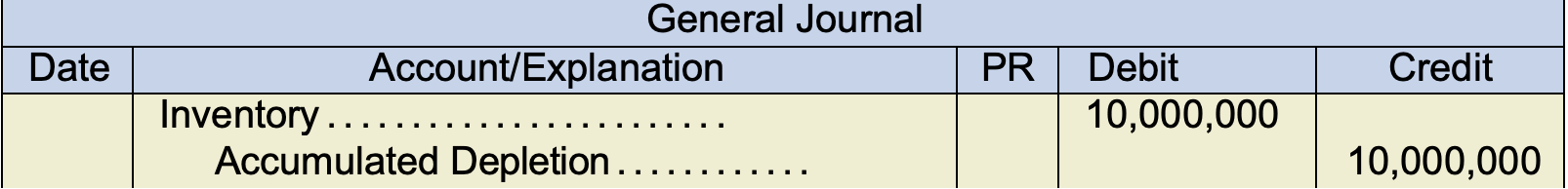
Note that in this case, inventory is impacted because this is an additional cost of the items that we want to sell. Remember that inventory ultimately flows through cost of goods sold.
10.2.4. Separate Components
As noted in Chapter 9, IFRS requires PPE assets be segregated into significant components. One of the reasons for doing this is that a significant component of the asset may have a different useful life than other parts of the asset. An airplane’s engine does not have the same useful life as the fuselage. It makes sense to segregate these components and charge depreciation separately, as this will provide a more accurate picture of the consumption of economic benefits from the use of the asset.
The process of determining what comprises a component requires some judgment from managers. A reasonable approach would be to first determine what constitutes a significant component of the whole and then determine which components have similar characteristics and patterns of use. Practical considerations, the availability of information, and cost versus benefit analyses (related to accounting costs) may all be relevant in determining how finely the components are defined. The goal is to create information that is meaningful for decision-making purposes without being overly burdensome to the company.
10.2.5. Partial Period Calculations
In the year of acquisition or disposal of a PPE asset, an additional calculation complication arises—namely, how to deal with depreciation for only part of a year. This occurs often since plant assets are rarely purchased on the first day of a fiscal period. There are several items to consider when purchasing a PPE asset throughout the fiscal year.
If the units-of- production method is being used to calculate depreciation expense, there isn’t a problem to calculate depreciation expense, since depreciation expense will be based on the actual production in the partial period. However, for time-based methods, like straight line or diminishing balance, an adjustment to the calculation of depreciation will be required.
Because accounting standards do not specify how to deal with this problem, companies have adopted a number of different practices. Although depreciation could be prorated on a daily basis, it is more usual to see companies prorate the calculation based on the nearest whole month that the asset was being used in the accounting period. Some companies will charge a full year of depreciation in the year of acquisition and none in the year of disposal, while other companies will reverse this pattern. Some companies charge half the normal rate in the years of acquisition and disposal. Whatever method is used, the total amount of depreciation charged over the life of the asset will be the same. As long as the method is applied consistently, there shouldn’t be material differences in the reported results.
As an example, assume that a piece of equipment with a five-year useful life is purchased for $30,000 (no residual value) on September 1, Y6. The company’s fiscal year end is December 31. The depreciation for this item, assuming straight-line depreciation would be: ($30,000 ÷ 5 years) × 4 ÷ 12 = $2,000 in Year 6. Watch the dates!
10.2.6. Revision of Depreciation
As noted previously, many elements of the depreciation calculation are based on estimates. IFRS requires that these estimates be reviewed on an annual basis for their reasonableness. If it turns out that the original estimate is no longer appropriate, how should the depreciation calculation be revised? The treatment of estimate changes re- quires prospective adjustment, which means that current and future periods are adjusted for the effect of the change. No adjustments should be made to depreciation amounts reported in prior periods. The reasoning behind this treatment is that estimates, by their nature, are subject to inaccuracies. As well, conditions may change; the asset may be used in a different fashion than originally intended, or the asset may lose function quicker or slower than originally anticipated. As long as the original estimate was reasonable in relation to the information available at the time, there is no need to adjust prior periods once conditions change.
Consider our original example of straight-line depreciation. The initial calculation resulted in an annual depreciation charge of $9,500. After two years of use, the company’s management noticed that the asset’s condition was deteriorating quicker than expected. The useful life of the asset was revised to seven years, and the residual value was reduced to $2,000. The revision to the depreciation charge would be calculated as follows:
(Remaining book value − Revised residual value) ÷ Remaining useful life
Thus, the calculation would be as follows:
($100,000 − ($9,500 × 2) − $2,000) ÷ (7 − 2 = 5 years remaining) = $15,800 per year
The company would begin charging this amount in the third year and would not revise the previous depreciation that was recorded. This technique is also applied if the company changes its method of depreciation, because it believes the new method better reflects the pattern of use or benefits derived from the asset, or if improvements are made to the asset that add to its capital cost.
- Note: In the final year, depreciation does not equal the calculated amount of net book value multiplied by depreciation percentage ($13,422 × 20% = $2,684). In the final year, the asset needs to be depreciated down to its residual value. The double-declining balance method will not result in precisely the right amount of depreciation being taken over the asset’s useful life. This means that the final year’s depreciation will need to be adjusted to bring the net book value to the residual value. Depending on the useful life of the asset, this final-year depreciation amount may by higher or lower than the amount calculated by simply applying the percentage. Because depreciation is an estimate based on a number of assumptions, this type of adjustment in the final year is considered appropriate. ↵
