9.4 Restoring Long-Run Macroeconomic Equilibrium

We have already seen that the aggregate demand curve shifts in response to a change in consumption, investment, government purchases, or net exports. The short-run aggregate supply curve shifts in response to changes in the prices of factors of production, the quantities of factors of production available, or technology. Now, we will see how the economy responds to a shift in aggregate demand or short-run aggregate supply. We will be able to distinguish the long-run response from the short-run response.

Shifts in Aggregate Demand

Suppose an economy is initially in equilibrium at potential output [latex]Y_P[/latex] as in Fig 9.10 and operating at full employment where real [latex]GDP=LRAS[/latex] (potential GDP).

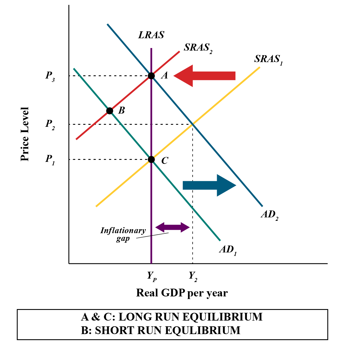
Suppose aggregate demand increases because one or more components (consumption, investment, government purchases, and net exports) have increased at each price level. For example, suppose consumption increases. The aggregate demand curve shifts from [latex]AD_1[/latex] to [latex]AD_2[/latex], as shown in Fig 9.10 above. That will increase real GDP to [latex]Y_2[/latex] and force the price level up to [latex]P_2[/latex] in the short run.

The economy’s new production level [latex]Y_2[/latex] exceeds potential output. Employment exceeds its natural level. The economy with output of [latex]Y_2[/latex] and price level of [latex]P_2[/latex] is only in short-run equilibrium; there is an inflationary gap equal to the difference between [latex]Y_2[/latex] and [latex]Y_P[/latex]. Because real GDP is above potential. At this level of output, the economy is overusing its resources and therefore resources tend to get costly. Ultimately, the nominal wage will rise as workers demand higher wages to keep overworking and producing more. As the nominal wage rises, the short-run aggregate supply curve will shift to the left because firms face increased labour costs. When the short-run aggregate supply curve reaches [latex]SRAS_2[/latex], the economy will have returned to its potential output, and employment will have returned to its natural level. These adjustments will close the inflationary gap. The price level rises to [latex]P_3[/latex] at the new equilibrium.

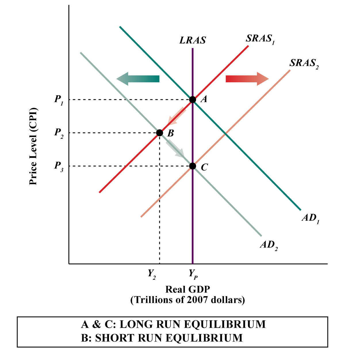
Suppose aggregate demand decreases because one or more components (consumption, investment, government purchases, and net exports) have decreased at each price level. For example, let us assume consumption decreases. The aggregate demand curve shifts from [latex]AD_1[/latex] to [latex]AD_2[/latex], as shown in Fig 9.11 above. That will decrease real GDP to [latex]Y_2[/latex] and force the price level to fall to [latex]P_2[/latex] in the short run.

The economy’s new production level [latex]Y_2[/latex] is less than the potential output. Employment is less than its natural level. The economy with output of [latex]Y_2[/latex] and price level of [latex]P_2[/latex] is only in short-run equilibrium; there is a recessionary gap equal to the difference between [latex]Y_2[/latex] and [latex]Y_P[/latex]. Because real GDP is less than potential, and unemployment tends to rise due to falling production. This could result in workers demanding less wages to retain jobs in such an economic crisis. As the nominal wage falls, the short-run aggregate supply curve will shift to the right because firms face decreased labour costs. When the short-run aggregate supply curve reaches [latex]SRAS_2[/latex], the economy will have returned to its potential output, and employment will have returned to its natural level. These adjustments will close the recessionary gap. The price level will fall to [latex]P3[/latex] at the new equilibrium.

Shift in Aggregate Supply (Supply Shock)

Again, suppose, with an aggregate demand curve at [latex]AD_1[/latex] and a short-run aggregate supply at [latex]SRAS_1[/latex], an economy is initially in equilibrium at its potential output [latex]Y_P[/latex], at a price level of [latex]P_1[/latex], as shown in Fig 9.12 below.

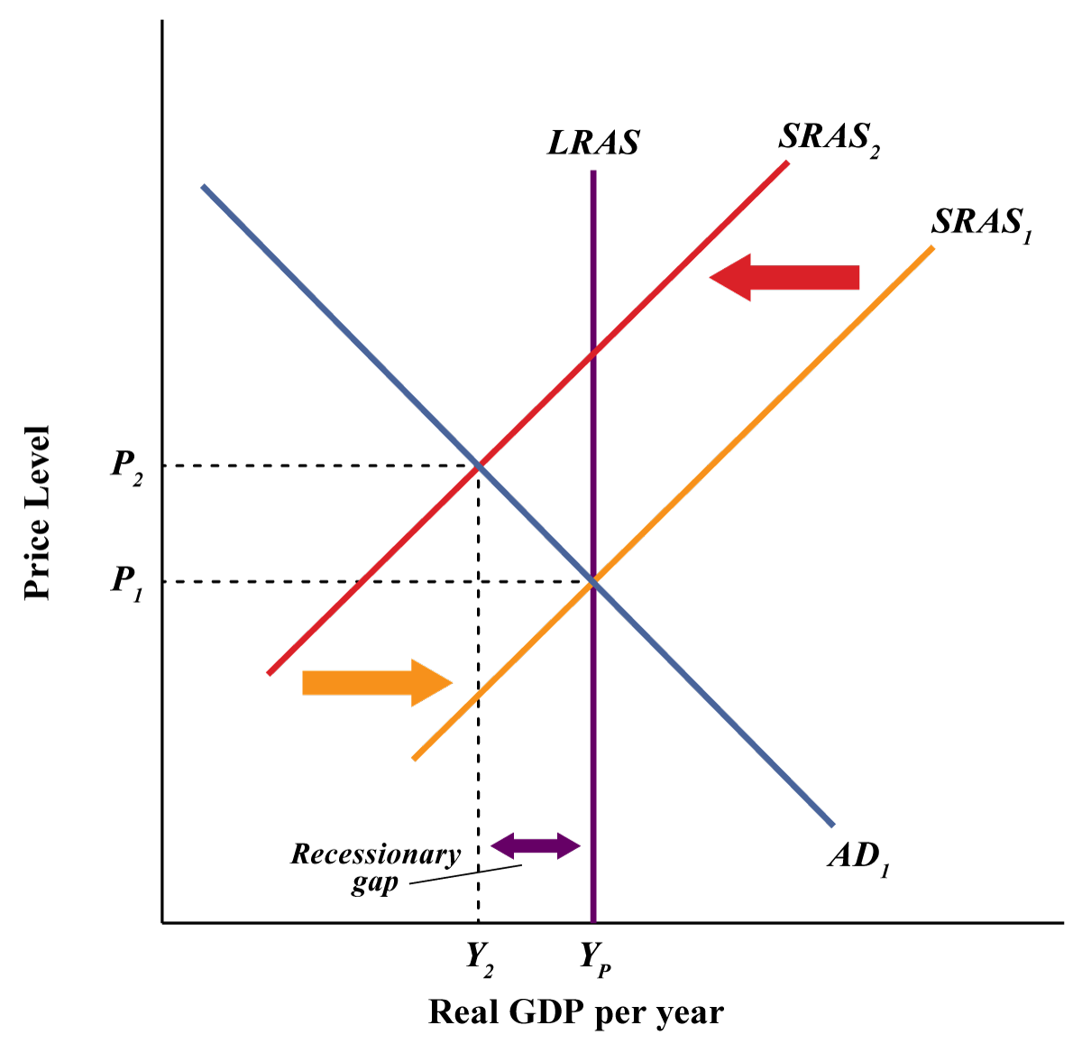
Now, suppose that the short-run aggregate supply curve shifts owing to a rise in the price of oil. This raises the cost of production and causes a reduction in the short-run aggregate supply curve from [latex]SRAS_1[/latex] to [latex]SRAS_2[/latex]. This decrease in the supply of oil is called a “supply shock.” A supply shock shifts the SRAS curve leftward.

As a result, the price level rises to [latex]P_2[/latex], and real GDP falls to [latex]Y_2[/latex]. The economy now has a recessionary gap equal to the difference between [latex]Y_P[/latex] and [latex]Y_2[/latex]. This is called stagflation. Stagflation is when the economy faces a decrease in real GDP and rising inflation.