2.3 Production Possibility Model

Just as individuals cannot have everything they want and must instead make choices, society as a whole cannot have everything it might want, either. This section of the chapter will explain the constraints society faces, using a model called the Production Possibilities Frontier (PPF).

In perspective

You are stranded on a tropical island alone. On this island, there are only two foods: pineapples and crabs.

In other words, you face a trade-off: any time you spend harvesting pineapples is time that cannot be spent looking for crabs. You are forced to decide on how to allocate the scarce resource of time.

 

While this is an extreme example, it is reflective of a common problem in production. Since there are only a certain number of hours in the day, time is a scarce resource. This scarcity limits the amount of total production.

Figure 2.2 displays a table showing several different combinations of goods that can be harvested in a given week. The table is very logical – if you spend all your time catching crabs, you will have no pineapples. Notice that you can produce either all crabs, all pineapples, or a mix of the two.

Assume you choose only to catch crabs. How many would have to be given up to obtain ten pineapples? In this example, three. This is an important concept; even though our scarce resource is time, we can measure the cost of a good, in this case, pineapples, in terms of the foregone good, in this case, crabs.

Notice how the marginal cost changes as you harvest more pineapples. To produce the next ten pineapples, it costs four crabs, and the following ten costs eight. Now, there are no more crabs to give up. While marginal opportunity cost is not continuously increasing, it is intuitive to think that the more pineapples you pick, the harder they will be to find, and therefore, the more time you will have to give up to harvest ten more.

In our example, while we would love to produce 30 pineapples and 30 crabs, this is out of our realm of possible production. In other words, it is not a point on our PPF.

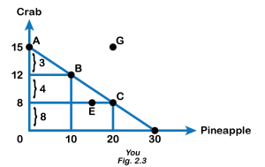
Using our terminology from before, each point along our PPF (i.e. Point A) is efficient (in a one-person world) since there is no way to get more pineapples without giving up some crabs and vice-versa. If we are inside the PPF (i.e. Point B), we are not fully using our resources. In this case, we can produce more pineapples without having to give up any more crabs. This point is inefficient. Points outside the PPF (i.e. Point C), while preferable, are unattainable given constraints in resources and time.

PPF and Increasing Opportunity Cost

Using our analysis of Marginal Cost (MC) from before, we see that the Slope (absolute value) of the PPF is the amount of the good on the vertical axis given up to obtain additional units of the good on the horizontal axis. Recall that the slope is calculated using rise overrun. From Fig 2.2, we see that to gain ten additional pineapples (from 10 to 20 units), we give up four crabs (12 to 8 units). To obtain another ten units of pineapples (from 20 to 30 units), we give up eight crabs (8 to 0 units) as we move down the PPF, the slope and MC increase. This pattern is common enough that economists have given it a name: the law of increasing opportunity cost.

This happens because some resources are better suited for producing certain goods and services instead of others. When the producer wants to obtain more pineapples and devotes more resources (time and effort) to it, there will be fewer resources available for obtaining the other goods, crab. Therefore, more pineapples result in the greater sacrifice of crabs.

Our government spends a certain amount of funds on reducing crime. However, additional increases typically cause relatively more significant increases in the opportunity cost of reducing crime and paying for enough police and security to reduce crime to nothing would be a tremendously high opportunity cost.

The curvature of the production possibilities frontier shows that as we add more resources to pineapples, moving from left to right along the horizontal axis, the original increase in opportunity cost is relatively small but gradually increases. In this way, the law of increasing opportunity cost produces the outward-bending shape of the production possibilities frontier.