9.3 Equilibrium in the AD-AS Model

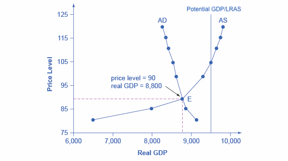
Figure 9.7 combines the short run [latex]AS[/latex] curve and the [latex]AD[/latex] curve from Figures 9.1 & 9.3 on the earlier pages and places them both on a single diagram. The intersection of the short-run aggregate supply and aggregate demand curves shows the equilibrium level of real GDP and the equilibrium price level in the economy. In this example, the equilibrium point occurs at point [latex]E[/latex], at a price level of [latex]90[/latex] and an output level of [latex]8,800[/latex]. This is called the short-run macro equilibrium.

Long-run macro equilibrium occurs when real GDP equals potential GDP. As discussed earlier, this is called the full employment level of output. At the long-run equilibrium, the short-run macro equilibrium point coincides with the potential GDP line. We will see this below.

Recessionary and Inflationary Gaps

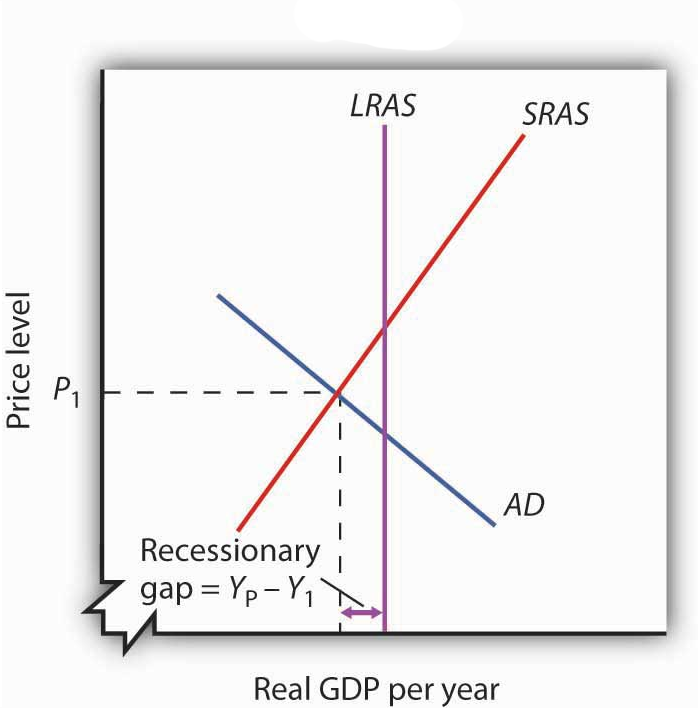
At any time, real GDP and the price level are determined by the intersection of the aggregate demand and short-run aggregate supply curves. If employment is below the natural level of employment, real GDP will be below potential. The aggregate demand and short-run aggregate supply curves will intersect to the left of the long-run aggregate supply curve.

The aggregate demand and short-run aggregate supply curves, [latex]AD[/latex] and [latex]SRAS[/latex], intersect to the left of the long-run aggregate supply curve [latex]LRAS[/latex] in Fig 9.8a. When real GDP is less than potential, the gap between real GDP and potential output is called a recessionary gap. The economy operates below its full employment level.

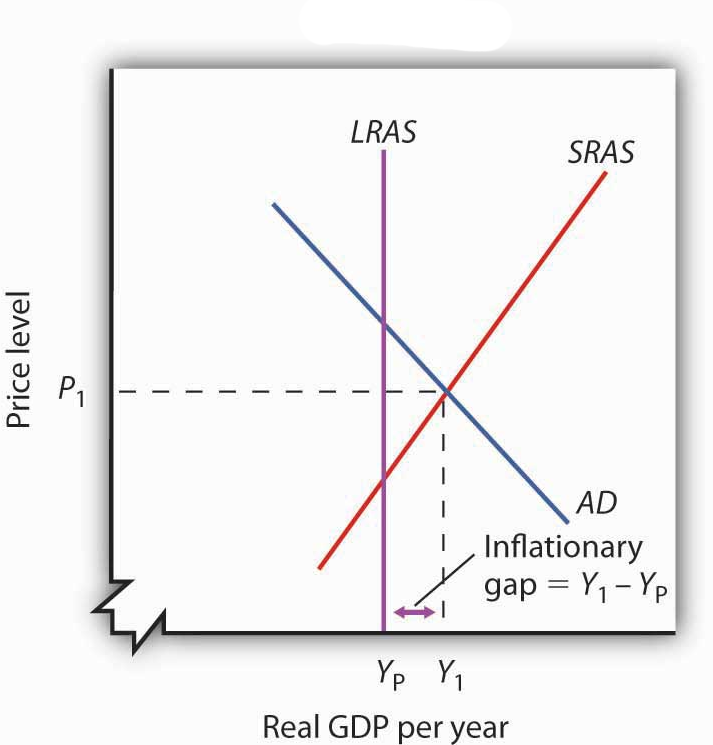
The aggregate demand and short-run aggregate supply curves, AD and SRAS, intersect to the right of the long-run aggregate supply curve LRAS in Fig 9.8b. The gap between the level of real GDP and potential output, when real GDP is greater than potential, is called an inflationary gap. The economy operates above its full employment level.

A recessionary or inflationary gap is referred to as an output gap in the Canadian economy. Output gaps are calculated as actual GDP less potential GDP as a percent of potential GDP.

Figure 9.9 plots the Bank of Canada’s estimates of the differences between actual and potential GDP for Canada, quarterly for each year from [latex]1992_{Q1}[/latex] to [latex]2019_{Q1}[/latex], expressed as a percentage of potential GDP.