8.2 The Components of Aggregate Expenditure

8.2.1 Consumption

Household consumption depends on several factors, such as:

• Disposable current and future income
• Household wealth
• The real interest rate
• Price levels

Keynes observed that consumption expenditure depends primarily on personal disposable income, i.e. one’s take-home pay. Let’s examine this relationship in more detail. People can do two things with their income: they can consume it, or they can save it. (For now, let’s ignore the need to pay taxes with some of it). Each person who receives a raise in income faces this choice. Let’s define the marginal propensity to consume (MPC) as the share (or percentage) of the additional income a person decides to consume (or spend). Similarly, the marginal propensity to save (MPS) is the share of the additional income the person chooses to save. Since the only options are to consume or save income, it must always hold true that:

[latex]\text{MPC}+\text{MPS}=1[/latex]

For example, if the marginal propensity to consume out of the marginal amount of income earned is 0.9, then the marginal propensity to save is 0.1.

Considering this relationship, consider the relationship among income, consumption, and savings shown in the table below.

To calculate the marginal propensity to consume,

[latex]\begin{align*}\text{MPC}=\frac{\text{Change in Consumption}}{\text{Change in Disposable Income}}\end{align*}[/latex]

A $1,000 increase in disposable income leads to an $800 increase in consumption, and then the MPC would be:

[latex]\begin{align*}\text{MPC}=\frac{800}{1,000}= 0.8\end{align*}[/latex]

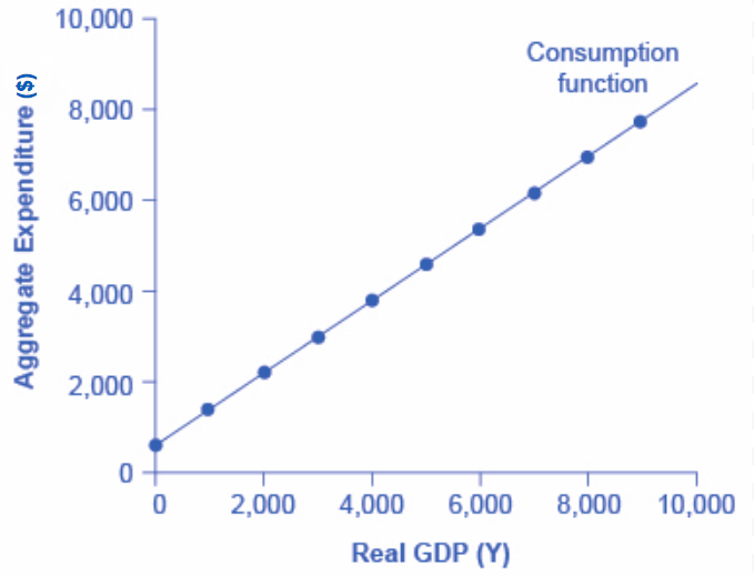
The consumption pattern shown in Fig 8.3 (table) is plotted in Fig 8.4. The relationship between income and consumption is called the consumption function. Both the table and figure illustrate a typical consumption function. There are a couple of features to observe. First, consumption expenditure increases as income does. For every increase in income, consumption increases by the MPC times that increase in income. Thus, the slope of the consumption function is the MPC. Second, at low levels of income, consumption is greater than income. Even if income were zero, people would have to consume something. We call the level of consumption when income is zero autonomous consumption since it shows the amount of consumption independent of income. In this example, consumption would be $600 even if income were zero. Thus, to calculate consumption at any income level, multiply the income level by 0.8 for the marginal propensity to consume and add $600 for the amount consumed even if income was zero.

Now, how does this relate to the national economy? For simplicity, we will re-write

[latex]\text{Disposable income}=\text{National income} - \text{Net Taxes}[/latex]

If we further re-write, we get

[latex]\text{National income}=\text{GDP}=\text{Disposable income}+\text{Net taxes}[/latex].

If we assume that net taxes will be constant based on a given income level (in reality, they are not, but let us keep this simple), then we see that any increase in national income will lead to an increase in consumption. The same holds for disposable income, as seen earlier.

Household Wealth

Wealth is defined as assets minus liabilities. Therefore, if the value of assets increases or the value of debt decreases, the household is wealthier. As household wealth increases, so will expenditure. Wealth can also encapsulate savings. A household with a larger safety net may be more likely to spend more knowing that if things go south, they can weather the storm. But, as wealth decreases, aggregate expenditure is likely to decrease as households cut spending and now has a smaller safety net.

Real Interest Rate

Spending on durable goods will likely be affected when the real interest rate changes. When purchasing a meal from a restaurant or hiring a lawyer, you rarely consider the interest rate. On the other hand, the interest rate will be important when purchasing a car or making some additional large purchases. Recall that the real interest rate is the difference between the nominal interest rate (what the bank charges you) and the inflation rate. As the real interest rate increases, the cost of borrowing will increase. This results in a decrease in aggregate expenditures as durable good purchases will fall. On the other hand, a decrease in the real interest rate makes it cheaper to borrow and will, therefore, increase aggregate expenditure, as people can increase their consumption.

Price Level

As the price of a single good increases, consumers will simply change how they spend their money on the good and will not affect overall spending. But, as the national price level changes, expenditure may change. If the average price level increases, goods and services are now more expensive. If disposable income remains constant, then $1 buys you less. Therefore, the total quantity of goods and services will fall. On the other hand, if price levels fall, a dollar becomes more valuable, meaning consumers can purchase more than before.

8.2.2 Planned Investment

Planned investment is determined by the following:

• Expectations of future profitability
• The real interest rate
• Taxes
• Cash flow

Expectation of Future Profitability

Investment does not yield immediate profit. Instead, investment requires a large upfront expenditure with the hope of earning future profits. But investment also requires a risk. Therefore, as firms expect greater future profitability, their appetite for investment risk will increase. Thus, an increase in expected future profit will lead to more investment while a decrease in expected future profit, such as during times of economic slowdown, will lead to a reduction in investment.

The Real Interest Rate

For the same rationale, as we saw with consumption, the real interest rate will dictate the cost of investment spending. Because investment can be costly, firms often must finance these investment activities. Again, the real interest rate gives the cost of borrowing. So, as the real interest rate increases, the borrowing cost increases, reducing investment spending. On the other hand, as the real interest rate decreases, the borrowing cost decreases, increasing investment spending.

Taxes

When considering consumption spending, we investigated income versus disposable income. While considering investment., we consider business or corporate taxes. If corporate taxes increase, companies must spend more on their tax payments and will, therefore, have less to spend on investment projects. But, if taxes fall, companies now have more money, all else equal, to spend on investment projects.

Cash Flow

While some companies finance their investment projects, others use cash to finance them. Therefore, the greater the cash flow for a company, the greater the ability to engage in these investment projects.

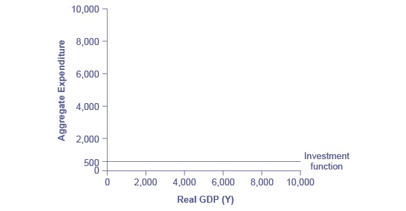
Just as a consumption function shows the relationship between real GDP (or national income) and consumption levels, the investment function shows the relationship between real GDP and investment levels. When businesses decide whether to build a new factory or place an order for new computer equipment, their decision is forward-looking, based on expected rates of return and the interest rate at which they can borrow for the investment expenditure. Investment decisions do not depend primarily on the current year’s GDP level. Thus, the investment function can be drawn as a horizontal line at a fixed level of expenditure. Because investment does not vary with real GDP, we call planned investment spending as autonomous.

8.2.3 Government Purchases

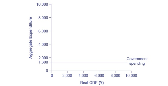
Federal, provincial, and local governments determine the level of government spending through the budget process. In the Keynesian aggregate expenditure model, government spending appears as a horizontal line, as in Figure 8.8, where government spending is set at $1,300 regardless of the level of GDP. As in the case of investment spending, this horizontal line does not mean that government spending is unchanging, only that it is independent of GDP. Like planned investment, G does not vary with real GDP, therefore, we call G or Government purchases as autonomous spending.

8.2.4 Net Exports

Exports are foreign purchases of domestically produced goods and services, meaning exports contribute to aggregate expenditure. Imports are purchases of foreign goods and services by domestic residents, which means that spending on imports takes away from spending on domestic goods and services. Let’s consider how imports and exports can be graphed as a function of national income (or real GDP).

We’ve established that consumption expenditure increases with national income; thus, in a macroeconomic context, the same thing is true of imports—the purchase of imports increases with national income. The foreign demand for our exports depends on their national income, but it is independent of our domestic national income. We can draw these two relationships as the export and import functions, shown below in Figures 8.9a and 8.9b.

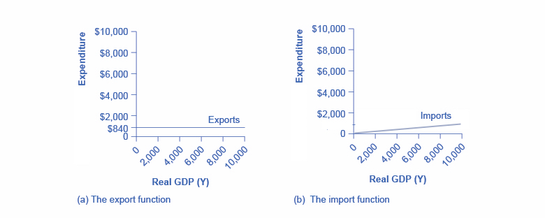
The export function, which shows how exports change with the level of a country’s real GDP, is drawn as a horizontal line, as in the example in Figure 8.9a, where exports are drawn at a level of $840. Again, as in the case of investment spending and government spending, drawing the export function as horizontal does not imply that exports never change. It means they do not depend on a country’s national income (or GDP). Therefore, export is also called autonomous spending, as exports do not vary with real GDP.

As explained above, the import function is an upward-sloping line, showing that as national income rises, so do import expenditures. The slope is given by the marginal propensity to import (MPI), which is the percentage change in import spending when national income changes. As real GDP increases, the country’s ability to import will likely go up. Import spending is induced, because just like consumption, imports vary with real GDP.

In Figure 8.9b, the marginal propensity to import is 0.1. Thus, if real GDP is $5,000, imports are $500; if real GDP is $6,000, imports are $600, and so on.