8.3 Putting It Together: The Aggregate Expenditure Function
The final step in deriving the aggregate expenditure function, which shows the total expenditures in the economy for each level of real GDP, is to sum the parts shown in Table 8.10.
| Real GDP | Consumption (C) | Investment (I) | Government Spending (G) | Exports (X) | Imports (M) | Net Exports (X-M) | Aggregate Expenditure (AE) |
|---|---|---|---|---|---|---|---|
| $0 | $600 | $500 | $1,300 | $840 | $0 | $840 | $3,240 |
| $1,000 | $1,160 | $500 | $1,300 | $840 | $100 | $740 | $3,700 |
| $2,000 | $1,720 | $500 | $1,300 | $840 | $200 | $640 | $4,160 |
| $3,000 | $2,280 | $500 | $1,300 | $840 | $300 | $540 | $4,620 |
| $4,000 | $2,840 | $500 | $1,300 | $840 | $400 | $440 | $5,080 |
| $5,000 | $3,400 | $500 | $1,300 | $840 | $500 | $340 | $5,540 |
| $6,000 | $3,960 | $500 | $1,300 | $840 | $600 | $240 | $6,000 |
| $7,000 | $4,520 | $500 | $1,300 | $840 | $700 | $140 | $6,460 |
| $8,000 | $5,080 | $500 | $1,300 | $840 | $800 | $40 | $6,920 |
| $9,000 | $5,640 | $500 | $1,300 | $840 | $900 | -$60 | $7,380 |
Graphically, the aggregate expenditure function is formed by adding (or stacking on top of each other) the consumption function (after taxes), the investment function, the government spending function, and the net export function. In its most basic form, the graph of aggregate expenditures looks like the graph shown in Fig 8.11.
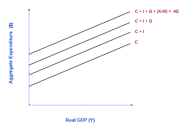
All the components of aggregate expenditure – consumption, investment, government spending, and net exports —are now in place to build the Keynesian cross diagram as shown below. The Keynesian cross diagram determines the equilibrium level of real GDP by the point where the total or aggregate expenditures in the economy are equal to the amount of output produced. The axes of the Keynesian cross diagram presented in Figure 8.12 show real GDP on the horizontal axis as a measure of output and aggregate expenditures on the vertical axis as a measure of spending. The 45-degree line illustrates that aggregate expenditure equals real GDP at every point on the line.
Note the vertical intercept of the aggregate expenditure function, that is, the point at which the aggregate expenditure function intersects the vertical axis is autonomous expenditure, i.e. all the components of aggregate expenditure (e.g. autonomous consumption, investment, government, and net export expenditures)—which do not vary with national income. The major part of consumption depends on national income, GDP, and imports. Therefore, consumption minus imports is called induced expenditure.
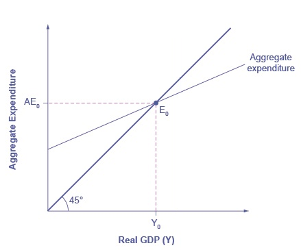
From Fig 8.12 above, the point where the aggregate expenditure line crosses the 45-degree line will be the equilibrium for the economy. It is the only point on the aggregate expenditure line where the total amount spent equals the total production level.
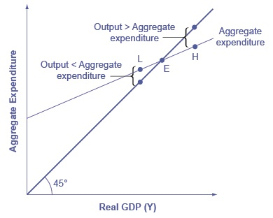
To understand why the point of intersection between the aggregate expenditure function and the 45-degree line is a macroeconomic equilibrium, consider what would happen if an economy found itself to the right of the equilibrium point E, say point H in Figure 8.13, where output is higher than the equilibrium. At point H, the level of aggregate expenditure is below the 45-degree line so that the level of aggregate expenditure in the economy is less than the level of output. As a result, output is piling up unsold inventories at point H — not a sustainable state of affairs.
Conversely, consider the situation where the level of output is at point L—where real output is lower than the equilibrium. In that case, the level of aggregate expenditure in the economy is above the 45-degree line, indicating that the level of aggregate expenditure is greater than the level of output. When the level of aggregate expenditure has emptied the store shelves, it cannot be sustained, either. Firms will respond by increasing their level of production. Thus, the equilibrium must be the point where the amount produced and the amount spent are balanced at the intersection of the aggregate expenditure function and the 45-degree line.
Attribution
“Aggregate Expenditure: Investment, Government Spending, and Net Exports” from Macroeconomics by Lumen Learning is licensed under a Creative Commons Attribution 4.0 International License.
“Chapter 9: The Aggregate Expenditure Model” in Introduction to Macroeconomics by J. Zachary Klingensmith is licensed under a Creative Commons Attribution-ShareAlike 4.0 International License.
