8.4 The Multiplier
Suppose that the macro equilibrium in an economy occurs where the economy is operating at full employment. Keynes pointed out that even though the economy starts at full employment, because aggregate expenditure tends to bounce around, it is unlikely that the economy will stay at full employment. In 2020, Canadian investment expenditure collapsed with Covid 19. As a result, the economy went into a Recession. But how much did GDP fall? Suppose investment fell by $100 billion. You might expect the result would be that GDP would fall by $100 billion, too. If so, you would be wrong. It turns out that changes in any category of expenditure have a more than proportional impact on GDP. Or, to say it differently, the change in GDP is a multiple of (say 3 times) the change in expenditure. This is the idea behind the multiplier.
For example, when businesses lower investments, they downsize and cut production. This, in turn, raises unemployment, and as income levels fall, people start cutting their consumption spending – the induced part. Therefore, aggregate expenditure decreases. So, the impact on the economy is much larger than the initial decrease in business investment. Real GDP decreases by more than the change in expenditure, which resulted from the investment cut.
What happens if there is an increase in Government purchases or the Government invests $200 million into opening a new EV plant in BC? We can see in Figure 8.15 that the curve shifts upward from the increase in [latex]\text{G}[/latex]. As G goes up. AE rises because G is a part of AE.
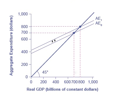
Changes in autonomous variables cause the [latex]\text{AE}[/latex] curve to shift vertically upward or downward. In this case, there is an increase in Government expenditure. So [latex]\text{AE}[/latex] curve shifts upward. We see there is a new equilibrium on the new [latex]\text{AE}[/latex] curve where [latex]\text{AE}_1[/latex] intersects with the 45-degree line. Even more important, the increase in real GDP is greater than the increase in [latex]\text{G}[/latex]. The multiplier effect we see in Fig 8.14 is explained below.

Suppose the government spontaneously purchases $100 billion worth of goods and services, perhaps because they feel optimistic about the future. The producers of those goods and services see an increase in income by that amount. They use that income to pay their bills, pay wages and salaries to their workers, rent to their landlords, and pay for the raw materials they use. Any income left over is profit, which becomes income to their stockholders. Each economic agent takes their new income and spends some of it. Those purchases then become new income to the sellers, who turn around and spend a portion of it. That spending becomes someone else’s income. The process continues, though, because economic agents spend only part of their income, the numbers get smaller in each round. The new income generated is multiple times the initial spending increase–hence, the spending multiplier. The table below shows how this could work with increased government spending. Note that the multiplier works the same way in reverse with a decrease in spending.
| Original increase in aggregate expenditure from government spending | 100 |
| Save 10% of income. Spend 90% of income. Second-round increase of… | 100−10=90 |
| $90 of income to people through the economy: Save 10% of income. Spend 90% of income. Third-round increase of… | 90−9=81 |
| $81 of income to people through the economy: Save 10% of income. Spend 90% of income. Fourth-round increase of… | 81−8.10=72.10 |
Fig 8.15 works through the process of the multiplier. Over the first four rounds of aggregate expenditures, the impact of the original increase in government spending of $100 creates a rise in aggregate expenditures of $100 + $80 + $60 + $40 = $280, which is larger than the initial increase in spending.
Fortunately, there is a formula for calculating the multiplier for everyone not carrying around a computer with a spreadsheet program to project the impact of an original increase in expenditures over 20, 50, or 100 rounds of spending.
- (a) [latex]\begin{align*}\text{Multiplier}=\frac{1}{(1-\text{MPC})}\end{align*}[/latex]
Suppose the [latex]\text{MPC}=90\%[/latex]; then the [latex]\text{MPS}=10\%[/latex]. Therefore, the multiplier is:
[latex]\begin{align*}\frac{1}{(1 - 0.9)}=\frac{1}{0.1}=10\end{align*}[/latex]
The second formula to calculate a multiplier is:
- (b) [latex]\frac{\text{Change in GDP}}{\text{change in any autonomous expenditure (I, G, or X)}}[/latex]
The multiplier applies when expenditure decreases as well as when it increases. Say that business confidence declines and investment (autonomous expenditure) falls off or that the economy of a leading trading partner slows down so that export (autonomous expenditure) sales decline. Because of the multiplier effect, these changes will reduce aggregate expenditures and have an even larger effect on real GDP.
Suppose a decrease in investment expenditure by $100 billion decreases GDP by $150 billion. The multiplier is: [latex]\frac{150}{100}=1.5[/latex], which implies GDP decreases by more than the initial fall in investment.
This chapter has looked at factors determining aggregate expenditure in the economy. In the next chapter, we can use the aggregate expenditure model to gain greater insight into understanding the aggregate demand model.
Attribution
“Chapter 9: The Aggregate Expenditure Model” in Introduction to Macroeconomics by J. Zachary Klingensmith is licensed under a Creative Commons Attribution-ShareAlike 4.0 International License.
