9.1 Aggregate Supply

The Aggregate Demand-Aggregate Supply model is designed to answer the questions of what determines the level of economic activity in the economy (i.e. what determines real GDP and employment) and what causes economic activity to speed up or slow down.

We can begin to answer these questions if we consider the aggregate production function concept, which we introduced in the context of economic growth. The aggregate production function shows the relationship between the resources (or factors of production) the economy has (e.g. labour, capital, technology, etc.) and the amount of output (i.e. real GDP) that can be produced. The resulting output is called Potential GDP if all resources are fully employed. (Over time, as the economy obtains more resources, the labour force and capital stock grow; as technology improves, the economy produces more GDP. We have described this process as economic growth.)

Firms decide what quantity of output to supply based on the profits they expect to earn. Profits, in turn, are also determined by the price of the outputs the firm sells and the price of the inputs, like labour or raw materials, the firm needs to buy.

Aggregate supply ([latex]AS[/latex]) refers to the total quantity of output (i.e. real GDP) firms will produce. The aggregate supply ([latex]AS[/latex]) curve shows the total quantity of output firms will produce and sell (i.e. real GDP) at each aggregate price level, holding the price of inputs fixed.

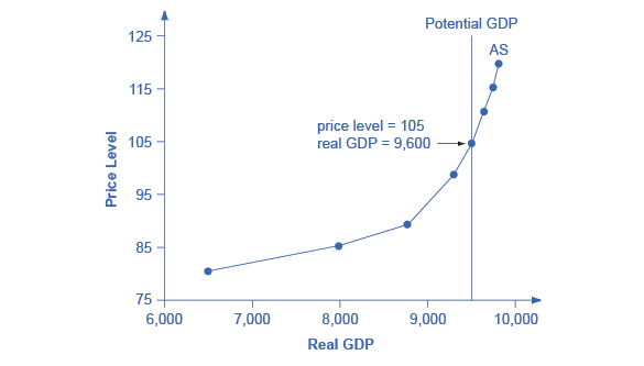
Recall that the aggregate price level is an average of the prices of outputs in the economy. Suppose we define the short run as the period of time that wages are sticky. In that case, we can describe the positive relationship between [latex]P[/latex] & [latex]Q[/latex] as the short-run aggregate supply ([latex]SRAS[/latex]) curve, shown above in Figure 9.1 as [latex]AS[/latex]. Aggregate supply ([latex]AS[/latex]) slopes up because as the price level for outputs rises, with the price of inputs remaining fixed, firms have an incentive to produce more and earn higher profits. The [latex]AS[/latex] curve describes how suppliers will react to a higher price level for outputs of goods and services while holding the prices of inputs like labour and energy constant.

If firms across the economy face a situation where the price level of what they produce and sell is rising, but their production costs are not rising, then the lure of higher profits will induce them to expand production.

A change in the price level produces a change in the aggregate quantity of goods and services supplied and is illustrated by the movement along the short-run aggregate supply curve, all else constant.

However, wages and prices are fully flexible in the long run. Consequently, all resources will be fully employed, and real GDP will equal potential, regardless of the price level. Thus, in the long run, real GDP will be independent of the price level, and the long-run aggregate supply ([latex]LRAS[/latex]) curve will be a vertical line at the potential (or the full employment level of) GDP. This can be seen in Fig 9.1 as potential GDP ([latex]PGDP[/latex]) or as [latex]LRAS[/latex]. Rather than prices, what affects or influences an economy’s growth potential would be the availability of resources, which we will discuss below and therefore, the LRAS is modelled as a vertical line, indicating that it is independent of the price level.

In Fig 9.1, at the far left of the aggregate supply curve, the level of output in the economy is far below the potential GDP. At these relatively low levels of output, levels of unemployment are high, and many factories are running only part-time or have closed their doors. The economy produces an output level where real GDP is less than potential GDP.

At the far right, the economy’s output level is higher than the potential GDP. The economy produces an output greater than the potential GDP. In this example, the vertical line in the exhibit shows that potential GDP occurs at a total output of 9,500. When an economy is operating at its potential GDP, machines and factories are running at capacity, and the unemployment rate is at its natural unemployment rate. For this reason, when real GDP equals potential GDP, we also call it full-employment GDP. That is, the economy operates at its capacity by fully employing its available resources.

Changes or Shifts in the Short Run Aggregate Supply Curve

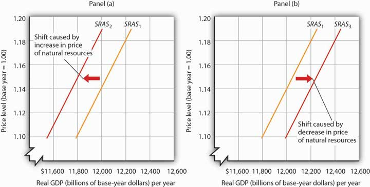
Changes in the factors held constant in drawing the short-run aggregate supply curve will shift the curve. An increase in capital stock, an increase in natural resources, technological advancement, or a fall in the prices of factors of production will shift the Aggregate Supply curve rightward.

Changes or Shifts in the Long Run Aggregate Supply Curve [latex]\left(\text{PGDP}\right)[/latex]

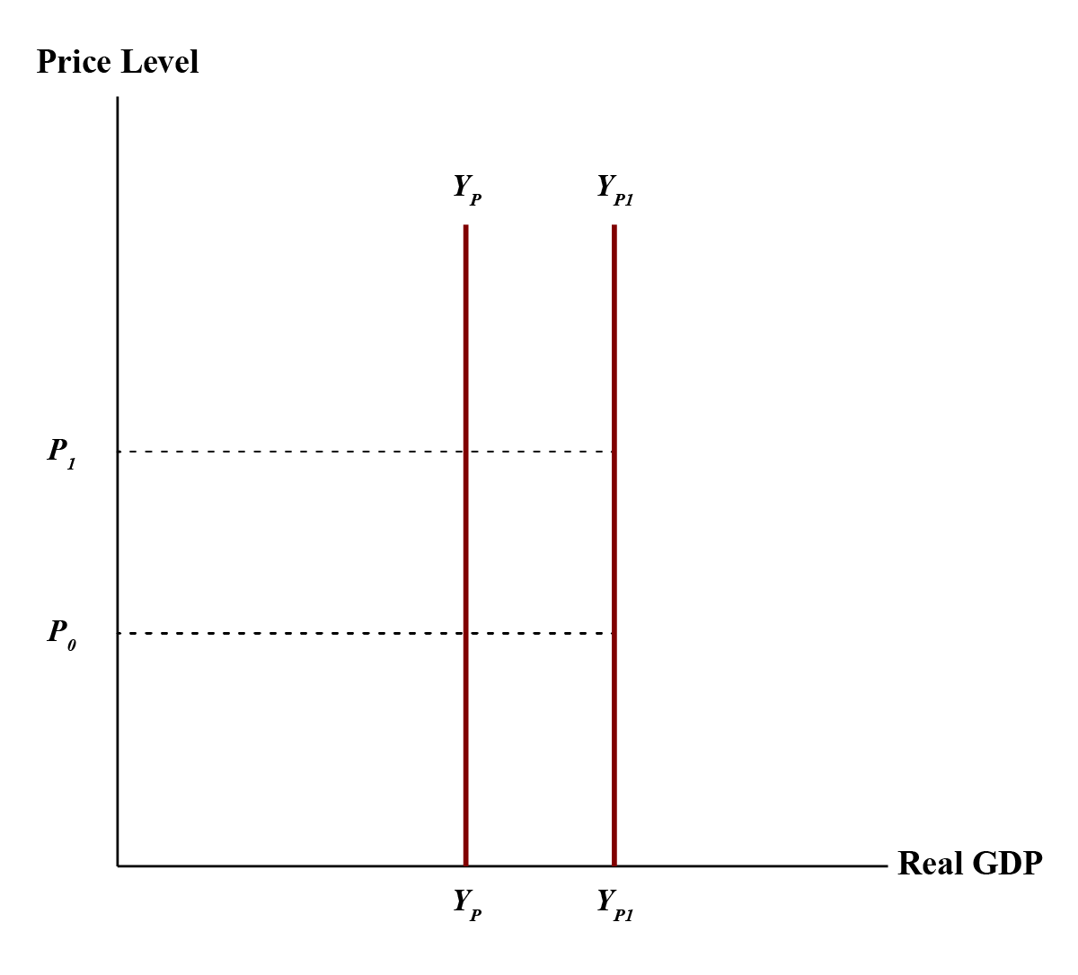
Growth in the labour force and improvements in labour productivity increase the economy’s potential GDP or potential output over time. Labour productivity grows due to advances in technology and investments in capital equipment, acquiring education and training. We see the increase in potential GDP in Fig 9.3 below. When labour becomes more productive, the demand for labour increases, and firms are willing to pay more for a given number of hours. This likely increases the output the economy produces because the same labour can now produce more goods and services, with growth in human capital and with the availability of physical capital and/or technology. A resourceful labour force is the outcome of greater educational qualifications, skills, and on-the-job training. Remember that human capital, physical capital, and technological advancements not only increase the economy’s growth potential but also enables the economy to produce more in the short run. In other words, the above factors would cause rightward shifts in the LRAS as well as the SRAS curves.