Chapter 8 Lab Overview and Background Information
Bradford Assay Learning Outcomes: Upon completion of this lab, students will gain practical experience in:
- Using a plate reader
- Making serial dilutions
- Performing a Bradford assay
Protein Quantification: Bradford Assay
You will continue on your DHFR protein purification journey by conducting a Bradford assay (1) to quantify the protein concentration in your samples. This is necessary in order for you to set up your protein crystal trays properly. It is important to know the exact amount of DHFR protein you will add to your protein crystals so that your results are reproducible. In this lab you will use the Bradford method to determine the concentration of the samples you saved from your Ni-NTA protein purification experiment. You will also use bovine serum albumin (BSA) as a standard protein.
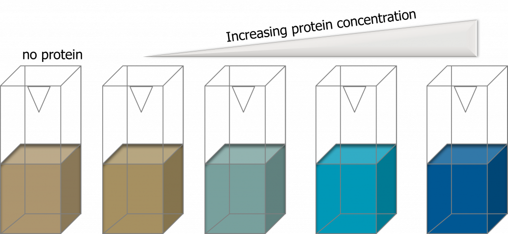
The Bradford (dye-binding) assay is based on the observation that the absorbance maximum for an acidic solution of the dye Coomassie Brilliant Blue G-250 shifts from 465 nm to 595 nm when binding (adsorption) to basic amino acids occurs. The absorbance increase at 595 nm is monitored and can be directly related to the amount of protein present (adapted from, (1), page 69). What does this mean in a practical sense? Your solution will turn from reddish/brown (little to no protein present) to a vibrant blue color (protein is present: the darker the blue color, the more protein you have in your reaction).
Advantages of the Bradford assay are: the stability of the dye-protein complex avoids the precise timing required for other methods. This assay, however, is subject to considerable protein-to-protein variation and non-linearity is often observed at high protein concentrations.
The Beer-Lambert Law
The Beer-Lambert law relates the difference in the intensity of incident light and transmitted light to the concentration of an absorbing chromophore in a given path length (2):
A = εbc, where A = Absorbance
ε = molar absorptivity (L*mol-1*cm-1)
b = path length (cm)
c = molar concentration (mol*L-1)
The linear relationship between absorbance (A) and concentration (c) breaks down when:
- The solution becomes very non-ideal (at high concentrations of chromophore)
- Chemical processes occur, such as side reactions (dissociation, association, solvolysis)
In this lab we will use both of these concepts to determine the concentration of total protein in our samples.
- We will add Coomassie Brilliant Blue dye to a small amount of each protein sample obtain from the Ni-NTA purification experiment.
- We will use a spectrophotometer (in the form of a microplate reader) to measure the absorbance at 595 nm. This measurement will allow us to determine the concentration of total protein in our samples by creating a standard curve which follows the linear relationship principle of the Beer-Lambert law (the linearity must be present in the standard curve otherwise we cannot directly correlate absorbance at 595 nm with concentration of protein). When plotting the values on the standard curve, you must ensure that you only use the linear portion of the curve to calculate your protein concentration. This relationship does not hold if your standard curve is not linear.
The equation of a line is as follows (2):
Y = mX + b
Where m = slope, and b = y-intercept
For your standard curve, the Y-axis is absorbance and the X-axis is concentration (or amount of your known protein samples). Therefore, the equation of the line is (2)
A = mC + b
Depending on the nature of data collection/analysis, the Y-intercept is normally zero due to the fact that at zero concentration of protein the instrument has been adjusted to an absorbance of zero OR your data has been adjusted to account for the background readings (such as your blank). Thus the equation of the line reads (2):
A = mC
So let’s look at this equation carefully. What determines the steepness of the slope? In some cases, the slope can be very steep indicating a dramatic absorbance change over a concentration range (2). In other cases, the slope may not be very steep. So obviously the nature of the analyte is a huge determining factor (2). The other main factor affecting the slope is the path length (the width of the cuvette holding the sample). If the light has to pass through a longer path, then there is more absorbing material present and more of the light will be absorbed (2). Thus the equation above can actually be written as A = εbC, bringing us back to the famous Beer-Lambert Law.
The BSA standard curve – Bovine Serum Albumin (BSA) will be used as your protein for creating a standard curve using the colorimetric Bradford assay. You will first need to serially dilute a stock concentration of BSA. A serial dilution is different from a regular dilution because it is a STEPWISE dilution of a substance in solution. For example, let’s say you have a 10 mg/mL solution of BSA and you need to make a dilution at a final concentration of 100 ng/mL. Your final volume is 1 mL. How do you make this dilution? Well, if you do the math, you have 100 ng = 0.1 µg = 0.0001 mg = 1 x 10⁻⁴ mg.
If we use:
CiVi = CfVf (whereby i= initial and f = final)
We have:
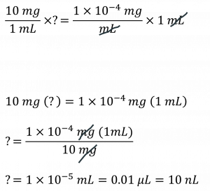
OK, now going back to your pipetting basics: what is the smallest volume you can accurately/precisely pipette? By our recollection it is 0.5 µL. That’s 500 nL and you need to measure 10 nL. See the problem? One way to get around this is to conduct a serial dilution. Let’s say final volume for each stepwise dilution is 1 mL and you will make 3, 1/10 dilutions. This means that from your stock of 10 mg/mL BSA you will conduct one dilution (1/10) to a final concentration of 1 mg/mL. Let’s calculate:
CiVi = CfVf

This means that you will take 100 µL of your 10 mg/mL BSA stock and add it to 900 µL solvent (in this case water) to make your final desired concentration of 1 mg/mL BSA (total volume of 1 mL)
Now repeat this process, only this time you ignore the 10 mg/mL BSA stock solution (it doesn’t exist as far as you’re concerned) and you use your newly created 1 mg/mL BSA solution as your new STOCK solution. You want another 1/10 dilution of this, so your final concentration will be 1/10 = 0.1 mg/mL BSA in a final volume of 1 mL. Let’s calculate:
CiVi = CfVf

This means that you will take 100 µL of your 1 mg/mL BSA stock and add it to 900 µL solvent (in this case water) to make your final desired concentration of 0.1 mg/mL BSA (total volume of 1 mL).
Are you starting to see a pattern? Now repeat this for the 3rd and final time, only this time you use 0.1 mg/mL as your stock. Let’s look at this in diagram form (much easier to see):
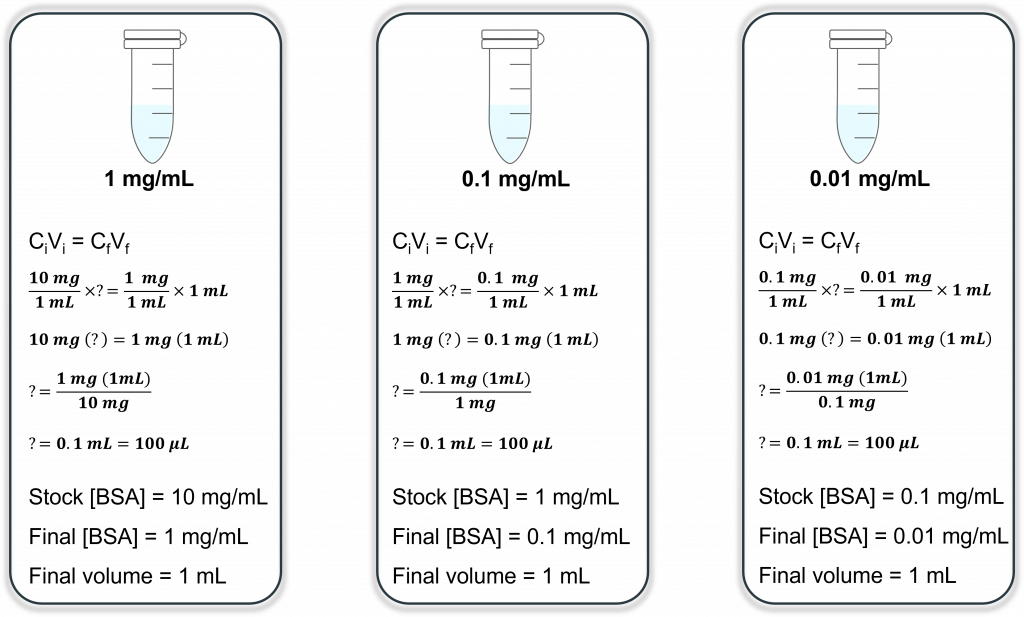
So your final dilution will have a final concentration of 0.01 mg/mL or 10 µg/mL. If we go back to our original problem (making 1 mL at a final [100 ng/mL]) we now need to add 10 µL of our 10 µg/mL stock (much more doable with our pipettes)!
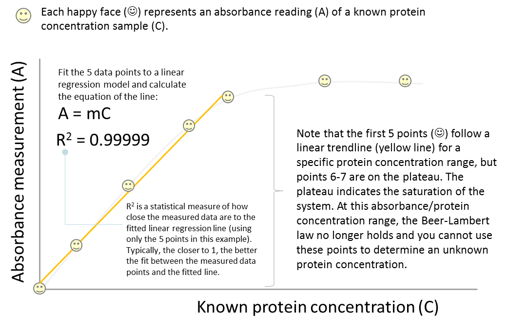
Once the BSA serial dilutions are made, Bradford reagent (aka. Coomassie dye) is added to a small sample of each known BSA concentration and incubated to allow for binding of the Coomassie dye to the protein, and color development. The absorbance at 595nm is measured for each sample using a spectrophotometer. The data is then plotted such that the BSA concentration is on the x-axis and the absorbance values on the y-axis. The test protein samples are then measured and the relative total protein concentration of the test samples is extrapolated from the linear part of the BSA standard curve:
In this lab we will be conducting the following BSA standard curve using a 96-well plate setup. The numbers in each well refer to the final BSA concentration in the well. Please note that each reaction is set up in triplicate to check for reproducibility. The colors reflect typical color development following addition of Bradford reagent and incubation.
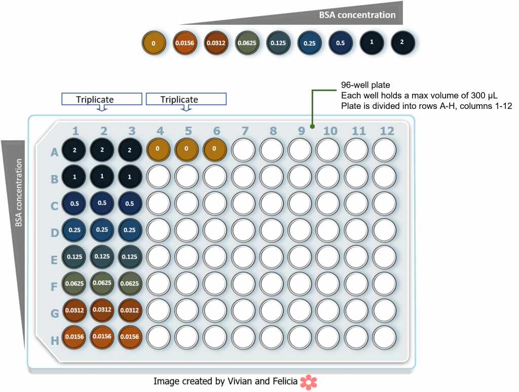
Following absorbance readings at 595 nm we should obtain the following data table:
| [BSA mg/mL] | Abs 595 (replica 1) | Abs 595 (replica 2) | Abs 595 (replica 3) |
| 2 | 1.129 | 1.029 | 0.987 |
| 1 | 1.012 | 0.987 | 1.031 |
| 0.5 | 0.757 | 0.665 | 0.762 |
| 0.25 | 0.510 | 0.476 | 0.554 |
| 0.125 | 0.363 | 0.327 | 0.380 |
| 0.0625 | 0.312 | 0.262 | 0.306 |
| 0.0312 | 0.272 | 0.258 | 0.274 |
| 0.0156 | 0.256 | 0.245 | 0.252 |
| 0 | 0.242 | 0.232 | 0.239 |
When reporting the final values, watch your significant digits. How many digits should you report before you lose confidence in the numbers you are reporting?
But what about the blank (0 BSA) absorbance value? This value is our background reading in the absence of any protein (quick tip: when measuring the absorbance values of your protein samples, any absorbance value equal or less than the blank absorbance value indicates the absence of protein in your sample).
One way to treat our current data set is to subtract the blank absorbance value from all our absorbance readings. To do this, simply subtract the average blank (0 BSA) value from every absorbance value for all your BSA samples (tip: you must also subtract this value from any other samples you test, such as your protein purification samples). The average 0 BSA absorbance value from the three replica samples equals 0.238. Subtracting 0.238 from all your absorbance readings yields the following.
| [BSA mg/mL] | Abs 595 (replica 1) | Abs 595 (replica 2) | Abs 595 (replica 3) |
| 2 | 0.891 | 0.791 | 0.749 |
| 1 | 0.774 | 0.749 | 0.793 |
| 0.5 | 0.519 | 0.427 | 0.524 |
| 0.25 | 0.272 | 0.238 | 0.316 |
| 0.125 | 0.125 | 0.089 | 0.142 |
| 0.0625 | 0.074 | 0.024 | 0.068 |
| 0.0312 | 0.034 | 0.020 | 0.036 |
| 0.0156 | 0.018 | 0.007 | 0.014 |
| 0 | 0.004 | -0.006 | 0.001 |
Next we need to calculate the average absorbance value for each BSA concentration, but we also need a way to report how precise the values are for each BSA concentration. Theoretically, all three absorbance values for each BSA concentration should be the same. However, in practice, lots of technical and experimental errors can occur so for each absorbance value we also need to report how close the values are to one another. To do this we calculate the standard deviation of all three absorbance values for each BSA sample and obtain the following:
| [BSA mg/mL] | Abs 595 (replica 1) | Abs. 595 (replica 2) | Abs. 595 (replica 3) | Average Abs. | St. Dev. |
| 2 | 0.891 | 0.791 | 0.749 | 0.811 | 0.073 |
| 1 | 0.774 | 0.749 | 0.793 | 0.772 | 0.022 |
| 0.5 | 0.519 | 0.427 | 0.524 | 0.490 | 0.055 |
| 0.25 | 0.272 | 0.238 | 0.316 | 0.276 | 0.039 |
| 0.125 | 0.125 | 0.089 | 0.142 | 0.119 | 0.027 |
| 0.0625 | 0.074 | 0.024 | 0.068 | 0.056 | 0.027 |
| 0.0312 | 0.034 | 0.020 | 0.036 | 0.030 | 0.009 |
| 0.0156 | 0.018 | 0.007 | 0.014 | 0.013 | 0.006 |
| 0 | 0.004 | -0.006 | 0.001 | 0.000 |
Graphing the average absorbance values (and calculated standard deviations) you will obtain the following graph (see below). You can then choose the linear part of the curve (this is the sensitivity range for your assay) and construct a linear trendline, complete with the equation of the line. You can use this equation to input your experimental absorbance values for all your unknown protein concentrations. This is what we mean when we talk about standard curves.
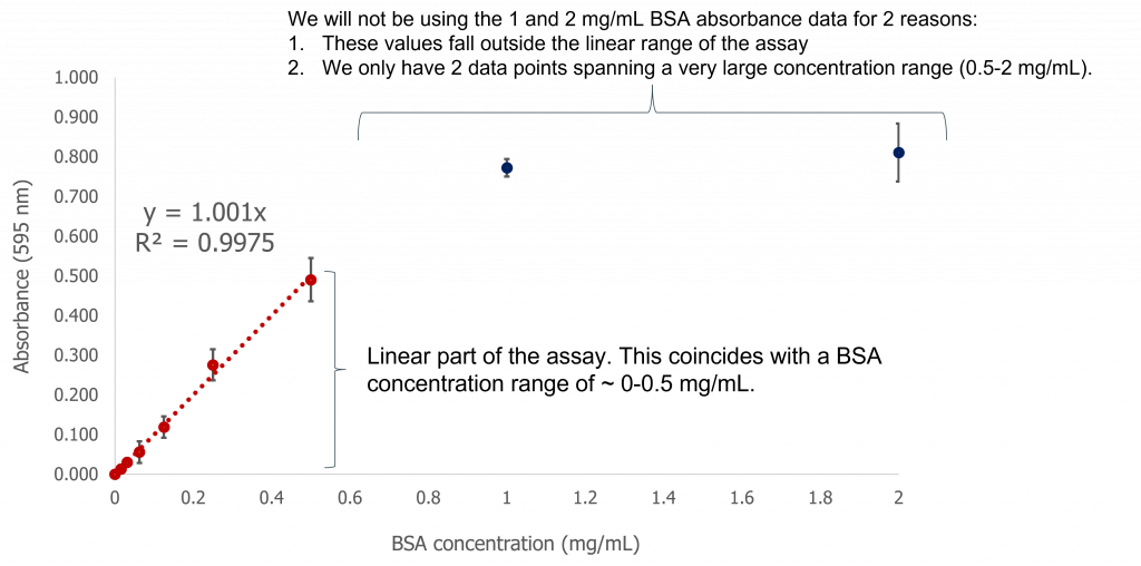
Image created by Felicia Vulcu using Microsoft Excel.
Equation of the line: Y=1.001X
R2 = 0.9975 (a measure of how closely your experimental data matches a linear relationship: the closer to 1, the more closely associated your data points are to a linear relationship).
