Chapter 1 Lab Overview and Background Information
Learning Outcomes: Upon completion of this lab, you will gain practical experience in:
- Calculating concentrations and amounts
- Pipetting accurately and precisely
- Solution making
- Amplifying DNA
- Setting-up a polymerase chain reaction experiment
This lab focuses on pipetting basics and PCR amplification of the E. coli folA gene.
- In Part A, pipetting basics, you will learn how to use micropipettes with accuracy and precision. You will also learn the basics of solution making.
- In Part B of this lab, you will design PCR primers (refer to the chapter “Think Tank 2” in Teaching Resources) and test these primers in your PCR. Your instructor will also design and optimize a set of primers that will be used as a positive control to PCR amplify your folA gene. You should always keep in mind why you are conducting this experiment. This step marks the beginning of your research project towards expressing, purifying, and characterizing your protein of interest; DHFR (Dihydrofolate Reductase).
This experimental plan is possible due to many scientific discoveries, some of which include:
1. Recombinant DNA cloning by Stanley Norman Cohen (and others) in 1973 (1).
2. Restriction endonucleases (aka. restriction enzymes) by Warner Arber, Daniel Nathans, and Hamilton Smith (2-7). These two discoveries led to the production of insulin, a true Canadian connection (8).
3. Discovery of PCR (Polymerase Chain Reaction) by Kari Mullis in 1983 (9-10). Other discoveries also helped build this field of Recombinant DNA Cloning (11).
4. Another great example is the identification of a bacterial plasmid by Joshua Lederberg in 1953 (Profiles in Science: The Joshua Lederberg Papers) (12).
Background information – Part A: Laboratory Basics: Pipetting and Preparing Solutions
Use of Pipettors
In Part A of this lab you will learn how to use a pipettor (also known as a micropipettor or pipette) to accurately measure and dispense small volumes of liquid. Pipettors are a common piece of equipment in a biochemistry lab and thus competence (and confidence!) in using them is an essential skill. You will have lots of practice using pipettors from this lab and throughout the course.
Proper use of a pipette is instrumental in ensuring experimental success. The majority of molecular biology deals with small volumes (less than 1000 μL). For example, your PCR reaction volume is a whopping 50 μL! This means that you must pipette all your reagents (DNA template, primers, polymerase, dNTPs, and buffer) in exact volumes to ensure success for your PCR. Pipetting mistakes will change the concentration of your reagents and therefore can result in no PCR amplicon (fun fact: an amplicon refers to a fragment of DNA that is the result of an amplification procedure). In your case, the DNA fragment containing your folA gene is known as the amplicon in your reaction. Thus, you need to master the art of pipetting such that you are both accurate and precise in your execution, so what do these two terms mean?
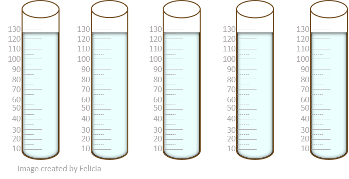
- Precision – “refers to the extent of agreement among repeated measurements of an experimental value”(13). It can also be described as reproducibility or repeatability (14). For example, say you want to pipette 125 μL of water in 5 different tubes. If you measure the volume of water in each tube and they all come out to 125 μL, then you can confidently say that you have 100% precision. It also gives you confidence in the calibration of your pipette in that it delivers reproducible results multiple times.
2. Accuracy – “is defined as the difference between the experimental value and the true value of the quantity” (13). Think about the example specified above. If you obtain the same result as above, but you programmed the pipette to dispense 75 μL you can say that your pipette’s accuracy is off by 50 μL (125 μL – 75 μL = 50 μL) but the precision (or reproducibility) is excellent. This could mean that your pipette is not calibrated accurately and is, therefore, a problem that you need to fix before using this pipette. Now, 50 μL might not seem like a large volume until you place this in context with your experiments. Again, remember your entire Polymerase Chain Reaction volume is 50 μL!
To calculate the accuracy (A) of our pipettes we can use the following equation:
![]()

![]()
If we were to expand this concept to the general scientific field, reproducibility is the key to making proper observations. We design our experiments such that we test a variable using a specific technique and our output is some form of measurement. We then process this measurement and analyze it by making correlations about its meaning as it pertains to our test hypothesis. But what about errors? How do they occur and how can we minimize them? Well, a lot of errors can be minimized using good laboratory practices (much like what you are doing with this pipetting exercise). In science we like to divide errors into 2 broad concepts:
1. Systematic error– “represented by a constant bias between your results and the true answer” (i.e. your equipment is not calibrated) this type of error can be eliminated using good laboratory practices (14).
2. Random error – “the result of random variations in experimental data”. This type of error is very difficult to control (14). Whenever possible we try to minimize the random error in our measurements. We often repeat our experiments more than one time (in fact, at least 3-6 times depending on the nature of the experiment) and we collect the sample size data. Typically we find the mean of this data as our reported output.
![]()
![]()
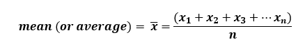
Whereby, x = individual values and n = number of observations
However, we also need to convey the reproducibility of our experiment and the mean does not give us this information. For example, we can have 3 data points with a mean of 2. The individual data points can be various number combinations. For example, they can all be 2, which would indicate high precision and reproducibility of our data. Alternatively, the mean can reflect a data set of 1, 2, and 3, which would indicate that we have a much lower reproducibility rate and a spread of 1 from the mean. Therefore, percent error and standard deviation calculations are used to determine the measure of accuracy and precision, respectively.
Whereby x= value of the sample, x bar = mean of the samples and n = number of samples.
Pipetting 101
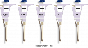
The following information on how to use a micropipettor has been adapted and modified from (15) and (16). Micropipettes (or pipettes) are air displacement pipettes used routinely in the research field to dispense small volumes (usually 0.5 µL – 1000 µL). They typically come in five sizes which are capable of pipetting five ranges of volumes: P10 =0.5-10 µL, P20 = 2- 20 µL, P100 = 10-100 µL, P200 = 20-200 µL and P1000 = 100-1000 µL. The pipettes require disposable plastic tips for use (16).
The following is an illustration of a Gilson micropipettor. You may also encounter Eppendorf and VWR pipettes which follow a similar design (16):
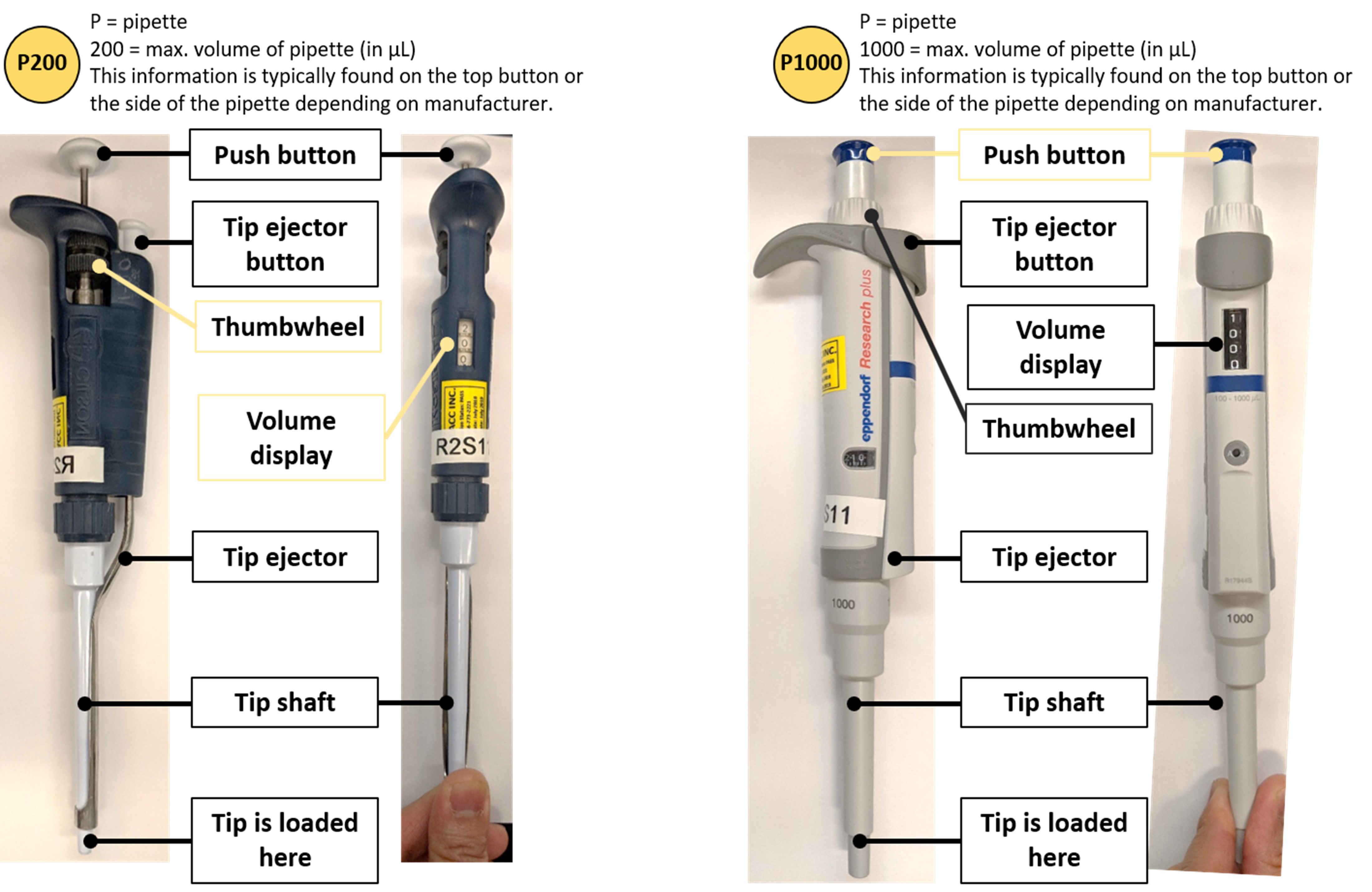
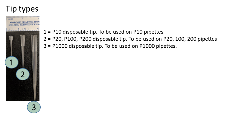
Figure 1: Parts of a pipette. Image made by Felicia. Pictures courtesy of Felicia Vulcu and Vivian Leong.
Now it’s your turn: please drag the appropriate pipette description to each of the four highlighted labels:
Pictures were taken by Felicia Vulcu, in collaboration with Vivian Leong.
Laboratory Calculations -some basic rules
And now it’s time to switch gears and go over some basic solution calculations. This section is extremely important and we will be using it for every single lab, so please spend some time and go over these general points and watch the corresponding e-content on this topic.
Please watch the following module to learn more about making solutions and performing calculations: Solutions and Dilutions Video
- A solution is a “homogenous mixture in which one or more substances is (are) dissolved in another. Solutes are the substances that are dissolved in a solution. The substance in which the solutes are dissolved is called the solvent.” (19).
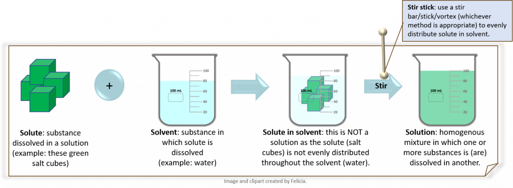
- Concentration is “ the amount of a particular substance (solute) in a stated volume (or mass) of a solution or mixture. Concentration is a RATIO where the numerator is the amount of material of interest and the denominator is usually the volume (or mass) of the ENTIRE mixture.” (19)
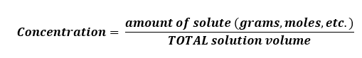
It is very important to keep in mind that concentration is a RATIO. Concentrations are the currency of most laboratory work as scientists typically report work in concentrations. This is because a concentration is very reproducible and it provides the scientists with a lot of information, namely the amount of a solute and the total solution volume. This is enough information to reproduce the solution.
For example, telling someone you made a salt solution of 1 gram/ 100 mL is very helpful. Telling someone you used 1 gram of salt in your experiments is wildly unhelpful and not reproducible at all. Please get into the habit of reporting laboratory information in the form of concentrations whenever possible.
The other important tip is to ALWAYS, ALWAYS include the units. Treat them almost like numbers and fractions. For example:
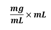
These are units, but watch what you can do with these if you treat them like typical fractions and apply basic arithmetic rules:
![]()
Super cool and awesome! Why? Because if you are ever in doubt of how to proceed with a calculation, you can obtain a ton of clues by following the units. Always follow the units.
Some basic formulas to keep in mind:
C1V1 = C2V2
Whereby C = concentration, V = volume, 1 and 2 refer to “stock” and “final, respectively
Tip: this equation only really works if you fully understand what you are trying to do in the lab.
Molarity: “equal to the number of moles of a solute that are dissolved per liter of solution, M = mol/L”. (19) Memorize this but also understand it. Do not confuse “M” with “mol or mole”. M is a concentration: mole/L (a ratio).
mole = 6.02 x 10²³ atoms (Avogadro’s number), however, some atoms are heavier than others therefore 1 mole of 1 element weighs a different amount than a mole of another element.
Weight of a mole of given element = atomic weight in grams or Gram Atomic Weight, see Periodic Table. Example: 1 mole carbon = 12.0 grams
By definition: a 1 Molar solution of a compound contains 1 mole of that compound dissolved in 1 Liter of the total solution.
The formula to use is: C = n/V, where C = concentration, n = number (e.g. in moles) and V = volume
Mass per Volume, where C = m/V (same as above except m = mass).
Percent Volume per Volume, such as 20 % (v/v). The designation % (v/v) describes the number of mL of liquid solute per 100 mL total volume. These units are used when the solute is a liquid such as glycerol or ethanol. Therefore, a 20 % (v/v) solution of glycerol implies 20 mL of glycerol in a total 100 mL solvent volume (in this example the solvent is water). To prepare this solution you would measure out 20 mL glycerol and add it to 80 mL water for a total of 100 mL.
Percent Weight per Volume, such as 20 % (w/v). The designation % (w/v) describes the number of grams of solute per 100 mL total volume. If you are asked to prepare a 25 % (w/v) solution you weigh out 25 grams of your solute and add it to your solvent (example, water) to a final total volume of 100 mL. Note that this makes the assumption that the added solute does NOT contribute significantly to the final volume.
However, this is not always the case so to ensure that your concentration is never prepared wrong add the solute to a volume of solvent (or water) that is LESS than the final volume, dissolve the solute, THEN add solvent (or water) to the final total volume.
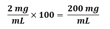
Fold Concentration, such as 100 X Buffer B. The “X” unit means that the concentration of each solute in this solution is a given number of times more concentrated than each is in a 1X solution. The usual assumption is that the final working solution is at a 1X concentration (although this is NOT always the case), irrespective of the units (mol/L, g/L, etc.). Thus, if a reagent should be at a final working concentration of 2 mg/mL and you need to make a 100X stock, you would use:
Things to note:
Keep in mind the units you are using and make sure you undergo appropriate inter-conversions. Many different types of concentration measurements can only be inter-converted between one another if additional information is available. For example: to convert from mg/mL to mM you need to know the molecular weight of the solute.
Dilution – “is when one substance (often but not always water) is added to another to reduce the concentration of the first substance. The original substance being diluted may be called the stock solution.” (19) For example, a 1 in 10 (or 1/10) dilution of a stock solution in a final volume of 10 mL means that you add 1mL of your stock solution to 9 mL water. (19)
Stock solution – concentrated solution, which you dilute prior to use
Working solution – diluted solution, ready to use
Dilution factor – is a dimensionless number that unambiguously describes the strength of the dilution. It is equal to the volume of the stock solution used divided by the total volume of the working solution produced. The dilution factor also gives the relationship between solute concentration in the stock solution and the working solution. (19)
Serial dilution – A sequential set of dilutions in which the stock for each dilution in the series is the working solution from the previous dilution.
Background – Part B: PCR amplification of your E. coli folA gene
Polymerase Chain Reaction (PCR)
The polymerase chain reaction (PCR) is an amazing technique that mimics the basic concepts of DNA replication. In this process, the 2 strands of the DNA double helix separate and act as templates for newly formed DNA.
This technique was successfully accomplished by Dr. Kari Mullis who received the Nobel Prize in 1993. The entire reaction depends on one key ingredient: a thermostable polymerase (enzyme). The enzyme must be thermostable as PCR relies on extreme temperature shifts to separate DNA strands allowing DNA primers to anneal and the polymerase to copy and produce new strands of DNA.
The main components of a PCR reaction are as follows:
– A thermostable polymerase (such as Taq DNA polymerase)
– dNTPs (monomeric building blocks for DNA: dCTP, dATP, dTTP, dGTP)
– DNA template (this can be any source of DNA, from genomic to plasmid, as long as it contains your gene of interest)
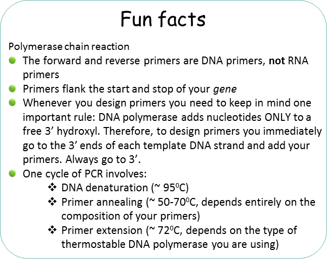
– Primers (this is a set of DNA primers that flank the start and end of your gene of interest). The primers are chemically generated oligonucleotides.
– Buffer (contains lots of really important things, like pH maintenance and Magnesium, which are required for a successful PCR)
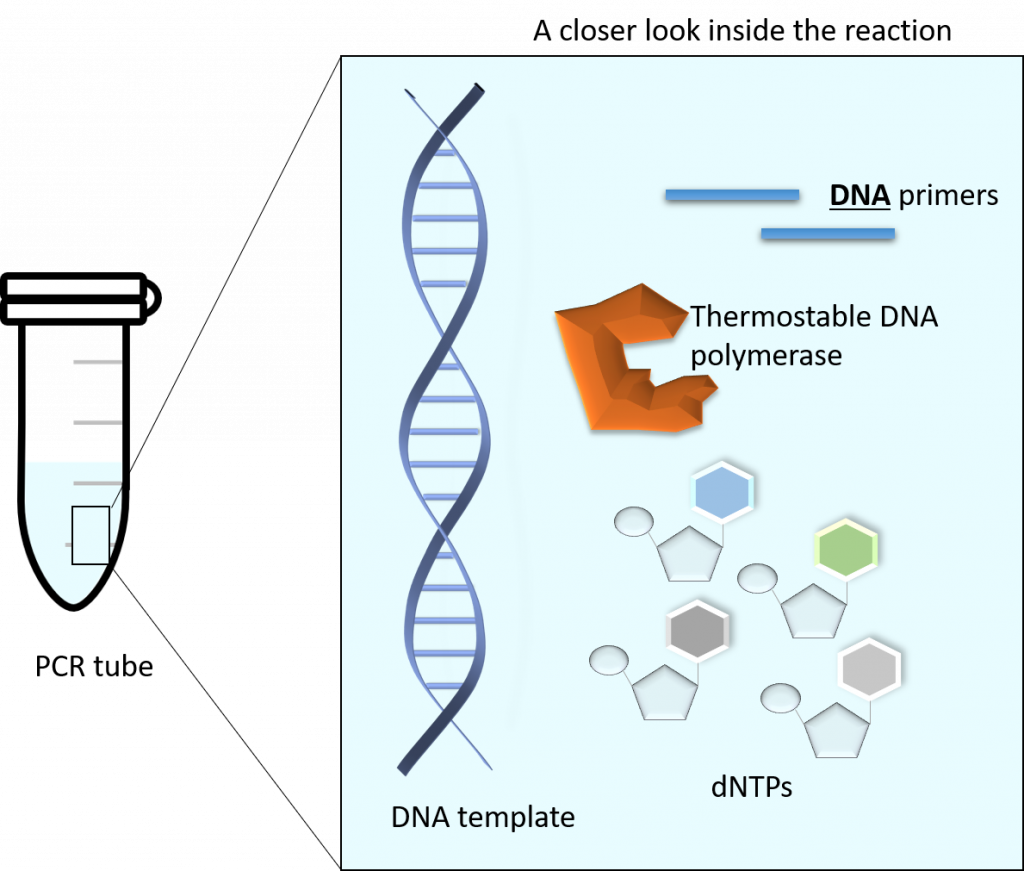
Image created by Felicia.
The entire reaction process can be described by these 3 temperature settings (note: some of these temperatures need to be optimized depending on the DNA to be amplified, and the type of thermostable polymerase used):
 95°C – (Denaturation step) “template” DNA is separated. In cellular DNA replication, this strand separation would be performed by enzymes. You can mimic this function using temperature in the PCR tube. By increasing the temperature to really high levels you can break down the hydrogen bonds that keep the two strands together.
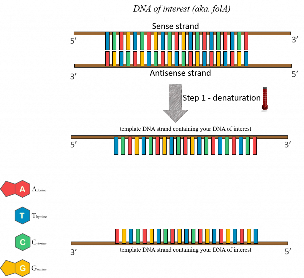
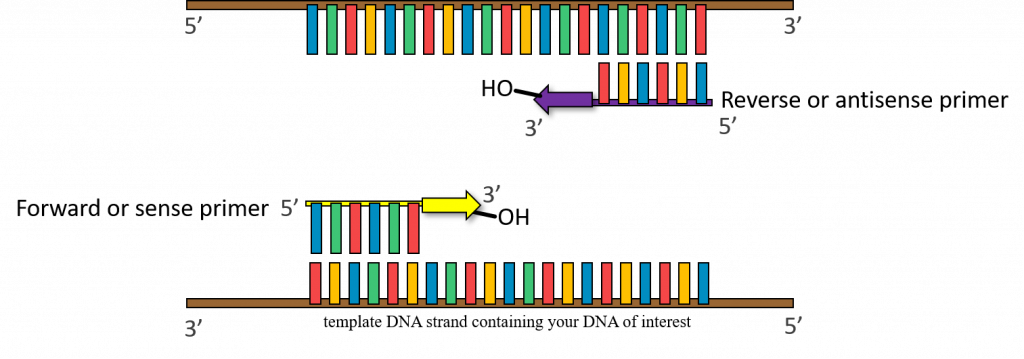
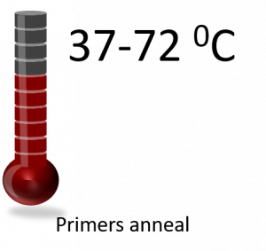 37-72°C – (Annealing step) oligonucleotide “primers” anneal to separated DNA strands. Annealing refers to the association of DNA primers to the complementary template due to hydrogen bonds that form between complementary base pairs. There are 2 primers, one complementary to the beginning of the DNA gene sequence to be amplified, and one complementary to the end of the DNA gene sequence to be amplified. In this way the primers flank the DNA sequence to be amplified! Please keep in mind that this reaction is taking place in a test tube and only borrows concepts of DNA replication. One very important distinction between PCR and cellular DNA replication is that in a polymerase chain reaction the primers are made of DNA.
 72°C – (Extension step) The thermostable DNA polymerase (such as Taq DNA polymerase) is now able to make copies of each strand starting from each annealed primer. This extension temperature can vary depending on the polymerase used.
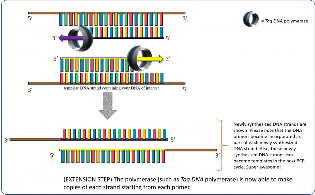
This cycle can be repeated for 24-30 cycles, doubling the number of copies of target DNA with each cycle giving us an exponential amplification. Assuming 100% efficiency, we can calculate the number of target DNA sequences at the end of the PCR cycle if we know the number of cycles and the number of copies of the target sequence initially present in the reaction:
![]()
Whereby N = number of copies after amplification, t = number of cycles, N₀ = number of copies initially present in the reaction
Putting this whole process together, we obtain the following PCR diagram:
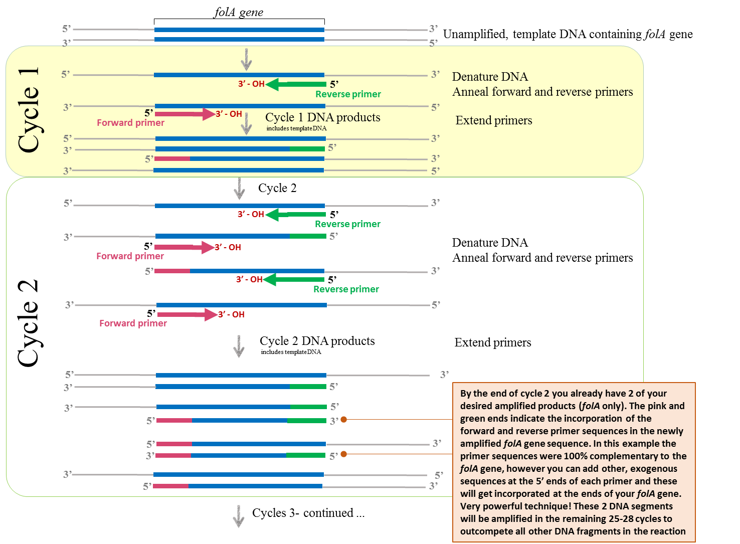
Figure 1 – Schematic diagram illustrating the concept of PCR. Image created by Felicia (loosely adapted from (22)
Please note that the unamplified, double-stranded DNA (containing your folA gene of interest) is first denatured (high heat) prior to the annealing of primers. The primers are complementary to each DNA strand and flank the beginning and end of your folA gene. The extension of the new DNA strand occurs from the free 3’ – OH end of each primer. Once annealed, the temperature is set for optimal extension of the primers to complete the new DNA strands. This step requires a thermostable DNA polymerase and dNTP’s (not shown in this figure). The cycle continues (denaturation, annealing, and extension) using the newly formed DNA strands as template DNA.
The Tm (melting temperature of primers) can be calculated for each primer using the following general formula:
![]()
The Tm of a pair of primers (forward and reverse) should be within a range of 1-4 degrees to ensure optimal PCR amplification. As a general rule-of-thumb, the Ta (annealing temperature of primers) is usually estimated to be 5 degrees below the Tm
![]()
These two equations are really important and you should commit them to memory. However, calculating annealing temperatures of primers is not solely dependent on the C/A/T/G composition, but also on the pH of the reaction, salts present, etc. These buffer conditions make a HUGE impact on the melting and annealing temperature. Nowadays, many companies that make and sell oligonucleotide primers also have their own, free primer annealing temperature calculators that mimic some of the real-world conditions in your reaction tube. It is important to keep in mind that these numbers are, at best, an educated guess to give you a starting point with respect to your first reaction conditions. Typically, when setting up PCR samples, you would test more than one condition to pinpoint the optimal reaction condition that yields a product. A couple of really good rules to follow are:
- Always understand what you are doing – know what you need to add to each tube and why each reagent is there.
- Always double-check that your primers are correct with respect to complementarity. Nowadays you can use many freeware computer programs for this task, but you can also ask a colleague to look over your gene sequence and your primer sequences to double, triple make sure.
- Use a computer program to determine your annealing temperature and try to use a program supplied by the company you will be ordering your primers from.
- Test more than one annealing temperature condition.
- Use a checklist when adding reagents to a PCR tube in order to ensure that you’ve added everything in the tube.
- Double, triple-check your reagents and the proper concentrations you need to add for each reagent.
|
Main Components of a Polymerase Chain Reaction Please note: the information in this table was compiled mainly from (26) Innis, M. A., Gelfand, D. H., Sninsky, J. J., & White, T. J. (Eds.). (2012). PCR protocols: a guide to methods and applications. Academic press.
|
|
|
Thermostable DNA polymerase (Taq DNA polymerase) |
Required to add dNTP’s to a growing strand of DNA during replication, standard concentration range for Taq DNA polymerase is between 1-2.5 units per 50 – 100 uL reaction |
|
MgCl2 |
Magnesium concentration may affect all of the following: primer annealing, strand dissociation temperatures of both template and PCR product, product specificity, formation of primer-dimer artifacts, enzyme activity and fidelity (26)
PCRs should contain 0.5-2.5 mM magnesium |
|
DNA template |
Contains your target gene to be amplified. In your case, you will be using plasmid DNA as your template DNA. Each plasmid DNA contains a copy of your gene of interest.
High DNA concentrations decrease amplicon specificity (i.e., extra bands on an agarose gel). |
|
Forward DNA primer The stock solution should be at 100 µM |
Final concentration between 0.1-0.5 mM (or around 20 pmol/primer)
Higher primer concentrations may promote mispriming and accumulation of nonspecific product and may increase the probability of generating a template-independent artifact termed a primer-dimer.
|
|
Reverse DNA primer |
Same as forward primer. |
|
Four dNTP’s |
Building blocks for replication. The 4 dNTPs should be used at equivalent concentrations to minimize mis-incorporation errors.
Optimal concentration: 20-200 µM each/reaction. |
|
Buffer components for PCR |
Typically 10-50 mM Tris-HCl (pH 8.3-8.8) is recommended for Taq DNA polymerase.
Up to 50 mM KCl can be included to facilitate primer annealing. NaCl at 50 mM or KCl above 50 mM inhibits Taq DNA polymerase activity. |