9.3 Single Monopoly Price and Output
Since a monopolist faces a downward-sloping demand curve, the only way it can sell more output is by reducing its price. Selling more output raises revenue, but lowering prices reduces it.
Let’s explore this using the data in the table in Fig 9.6, which shows quantities along the demand curve and the price at each quantity demanded and then calculates total revenue by multiplying price times quantity at each level of output. (In this example, we give the output as 1, 2, 3, 4, and so on, for the sake of simplicity. As the figure illustrates, total revenue for a monopolist has the shape of a hill, first rising, next flattening out, and then falling. In this example, total revenue is highest at a quantity of 6 or 7.
| Quantity Q |
Price P |
Total Revenue TR |
Total Cost TC |
|---|---|---|---|
| 1 | 1,200 | 1,200 | 500 |
| 2 | 1,100 | 2,200 | 750 |
| 3 | 1,000 | 3,000 | 1,000 |
| 4 | 900 | 3,600 | 1,250 |
| 5 | 800 | 4,000 | 1,650 |
| 6 | 700 | 4,200 | 2,500 |
| 7 | 600 | 4,200 | 4,000 |
| 8 | 500 | 4,000 | 6,400 |
Fig 9.6
However, the monopolist is not seeking to maximize revenue, but instead to earn the highest possible profit. In the Health Pill example, the highest profit will occur at the quantity where total revenue is the farthest above total cost.
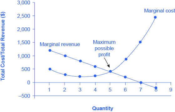
A monopolist can determine its profit-maximizing price and quantity by analyzing the marginal revenue and marginal costs of producing an extra unit. If the marginal revenue exceeds the marginal cost, then the firm should produce the extra unit.
For example, at an output of 4 in Fig 9.7, marginal revenue is 600 and marginal cost is 250, so producing this unit will clearly add to overall profits. At an output of 5, marginal revenue is 400 and marginal cost is 400, so producing this unit still means overall profits are unchanged. However, expanding output from 5 to 6 would involve a marginal revenue of 200 and a marginal cost of 850, so the sixth unit would actually reduce profits. Thus, the monopoly can tell from the marginal revenue and marginal cost that of the choices in the table, the profit-maximizing level of output is 5.
| Quantity Q |
Total Revenue TR |
Marginal Revenue MR |
Total Cost TC |
Marginal Cost MC |
|---|---|---|---|---|
| 1 | 1,200 | 1,200 | 500 | 500 |
| 2 | 2,200 | 1,000 | 775 | 275 |
| 3 | 3,000 | 800 | 1,000 | 225 |
| 4 | 3,600 | 600 | 1,250 | 250 |
| 5 | 4,000 | 400 | 1,650 | 400 |
| 6 | 4,200 | 200 | 2,500 | 850 |
| 7 | 4,200 | 0 | 4,000 | 1,500 |
| 8 | 4,000 | -200 | 6,400 | 2,400 |
Fig 9.8
Thus, a profit-maximizing monopoly should follow the rule of producing up to the quantity where marginal revenue is equal to marginal cost—that is, MR = MC. This quantity is easy to identify graphically, where MR and MC intersect, as shown in Fig 9.9.
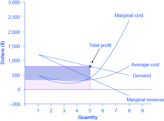
Fig 9.9 illustrates the three-step process where a monopolist: selects the profit-maximizing quantity to produce; decides what price to charge; determines total revenue, total cost, and profit.
The Monopolist determines its Profit-Maximizing level of output
The firm can use the points on the demand curve D to calculate total revenue, and then, based on total revenue, calculate its marginal revenue curve. The profit-maximizing quantity will occur where MR = MC — or at the last possible point before marginal costs start exceeding marginal revenue. In Fig 9.9, MR = MC occurs at an output of 5.
The Monopolist decides what price to charge
The monopolist will charge what the market is willing to pay. A dotted line drawn straight up from the profit-maximizing quantity to the demand curve shows the profit-maximizing price which, in Fig 9.9, price is $800. This price is above the average cost curve, which shows that the firm is earning profits.
Calculate Total Revenue, Total Cost, and Profit
Total revenue is the overall shaded box, where the width of the box is the quantity sold and the height is the price. In Fig 9.9, this is 5 × $800 = $4000. In Fig 9.9, the bottom part of the shaded box, which is shaded more lightly, shows total costs; that is, quantity on the horizontal axis multiplied by average cost on the vertical axis or 5 × $330 = $1650. The larger box of total revenues minus the smaller box of total costs will equal profits, which the darkly shaded box shows. Using the numbers, the profit earned is $4000 – $1650 = $2350.
Attribution
“8.1 Monopoly” in Principles of Microeconomics by Dr. Emma Hutchinson, University of Victoria is licensed under a Creative Commons Attribution 4.0 International License, except where otherwise noted.
“9.2 How a Profit-Maximizing Monopoly Chooses Output and Price” in Principles of Economics 2e by OpenStax is licensed under Creative Commons Attribution 4.0 International License.
