8.3 Comparing Marginal Revenue and Marginal Costs
The approach that we described in the previous section, using total revenue and total cost, is not the only approach to determining the profit-maximizing level of output. In this section, we provide an alternative approach that uses marginal revenue and marginal cost.
Firms often do not have the necessary data they need to draw a complete total cost curve for all levels of production. They cannot be sure of what total costs would look like if they, say, doubled production or cut production in half because they have not tried it. Instead, firms experiment. They produce a slightly greater or lower quantity and observe how it affects profits. In economic terms, this practical approach to maximizing profits means examining how changes in production affect marginal revenue and marginal cost.
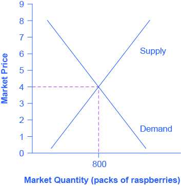
Fig 8.5 presents the marginal revenue and marginal cost curves based on the total revenue and total cost in Fig 8.2. The marginal revenue curve shows the additional revenue gained from selling one more unit. As mentioned before, a firm in perfect competition faces a perfectly elastic demand curve for its product—that is, the firm’s demand curve is a horizontal line drawn at the market price level. This also means that the firm’s marginal revenue curve is the same as the firm’s demand curve: Every time a consumer demands one more unit, the firm sells one more unit and revenue increases by exactly the same amount equal to the market price. In this example, every time the firm sells a pack of frozen raspberries, the firm’s revenue increases by $4. Fig 8.4 shows an example of this. This condition only holds for price-taking firms in a perfect competition where:
Marginal Revenue = Price
The formula for marginal revenue is:
Marginal Revenue = change in total revenue ÷ change in quantity
| Price | Quantity | Total Revenue | Marginal Revenue |
|---|---|---|---|
| $4 | 1 | $4 | - |
| $4 | 2 | $8 | $4 |
| $4 | 3 | $12 | $4 |
| $4 | 4 | $16 | $4 |
Fig 8.4
Notice that marginal revenue does not change as the firm produces more output. That is because, under perfect competition, the price is determined through the interaction of supply and demand in the market as shown in Fig 8.5, and does not change as the farmer produces more.
Since a perfectly competitive firm is a price taker, it can sell whatever quantity it wishes at the market-determined price. We calculate marginal cost, the cost per additional unit sold, by dividing the change in total cost by the change in quantity.
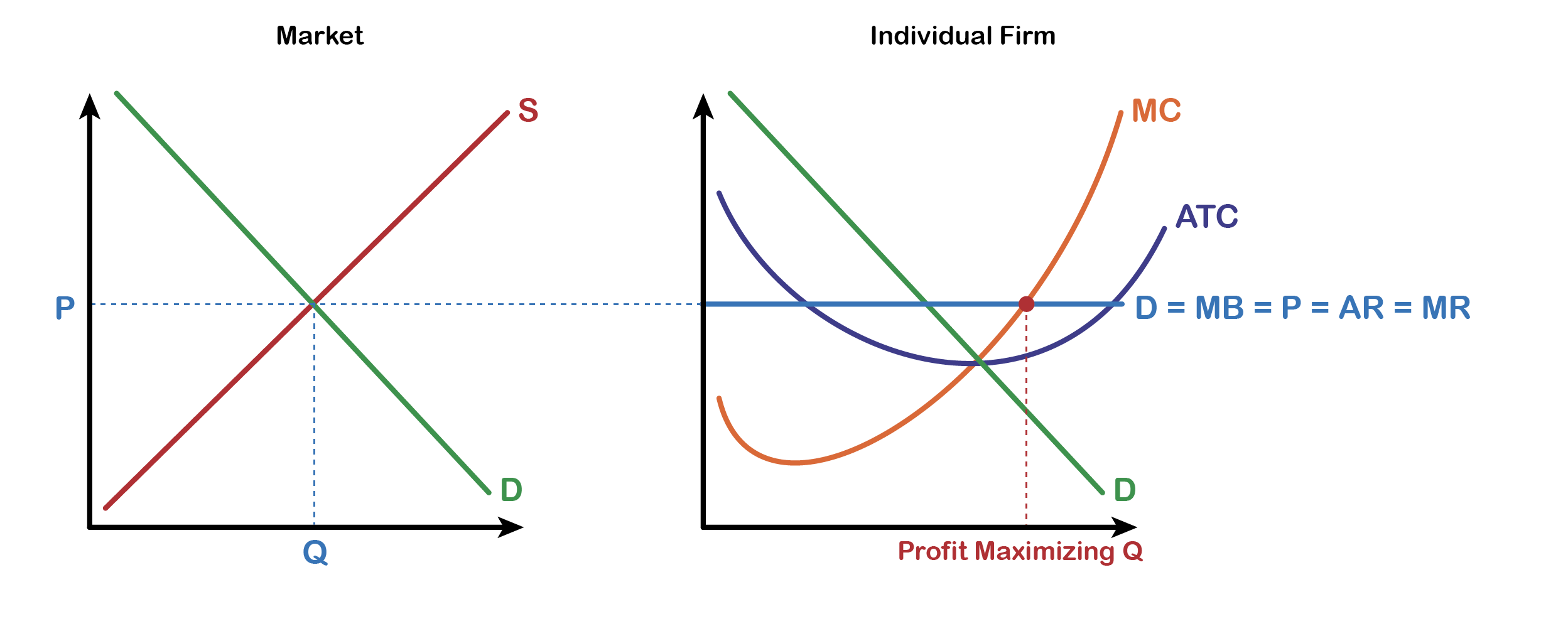
The figure above shows the market graph on the left panel (just as the example in Fig 8.5). Markets determine the price, and this is the price the perfectly competitive producer is charging. The right panel shows the price line which is also the perfectly elastic demand faced by a representative producer. The price and the demand is the marginal revenue earned by the producer for every additional unit of the good sold. The profit maximizing output produced is determined where the marginal revenue line intersects the marginal cost curve.
The formula for marginal cost is:
Marginal cost = change in total cost/change in quantity
Example
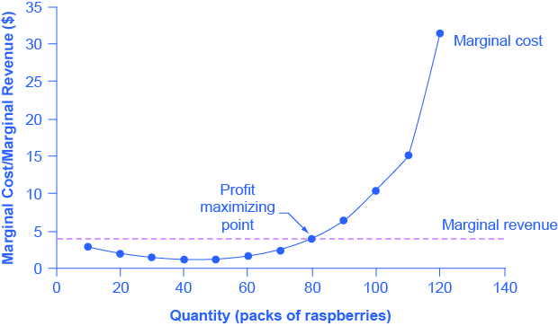
From Fig 8.6, if the firm is producing at a quantity where MR > MC, like 60 packs of raspberries, then it can increase profit by increasing output because the marginal revenue is exceeding the marginal cost. The revenue from the 60th pack more than compensates for the cost of producing the 60th pack of raspberry. If the firm is producing at a quantity where MC > MR, like 100 packs, then it can increase profit by reducing output because the cost of producing the 100th pack exceeds the revenue obtained from selling the 100th pack. The firm’s profit-maximizing choice of output will occur where MR = MC (i.e. at a quantity of 80 packs). The revenue obtained from selling the 80th pack of raspberry just compensates for the cost of producing the 80th pack.
The profit-maximizing choice for a perfectly competitive firm will occur at the level of output where marginal revenue is equal to marginal cost—that is, where MR = MC. This occurs at Q = 80 in Fig 8.7 below.
| Quantity | Total Cost | Marginal Cost | Total Revenue | Marginal Revenue | Profit |
|---|---|---|---|---|---|
| 0 | $62 | - | $0 | $4 | -$62 |
| 10 | $90 | $2.80 | $40 | $4 | -$50 |
| 20 | $110 | $2.00 | $80 | $4 | -$30 |
| 30 | $126 | $1.60 | $120 | $4 | -$6 |
| 40 | $138 | $1.20 | $160 | $4 | $22 |
| 50 | $150 | $1.20 | $200 | $4 | $50 |
| 60 | $165 | $1.50 | $240 | $4 | $75 |
| 70 | $190 | $2.50 | $280 | $4 | $90 |
| 80 | $230 | $4.00 | $320 | $4 | $90 |
| 90 | $296 | $6.60 | $360 | $4 | $64 |
| 100 | $400 | $10.40 | $400 | $4 | $0 |
| 110 | $550 | $15.00 | $440 | $4 | -$110 |
| 120 | $715 | $16.50 | $480 | $4 | -$235 |
Fig 8.7
Attribution
“8.2 How Perfectly Competitive Firms Make Output Decisions” in Principles of Economics 2e by OpenStax is licensed under Creative Commons Attribution 4.0 International License.
