6.3 Price Elasticity of Demand and Total Revenue
Example
Imagine that a band on tour is playing in an indoor arena with 15,000 seats. To keep this example simple, assume that the band keeps all the money from ticket sales. Assume further that the band pays the costs for its appearance, but that these costs, like travel, and setting up the stage, are the same regardless of how many people are in the audience. Finally, assume that all the tickets have the same price. The band knows that it faces a downward-sloping demand curve; that is, if the band raises the ticket price, it will sell fewer seats. How should the band set the ticket price to generate the most total revenue, which in this example, because costs are fixed, will also mean the highest profits for the band? Should the band sell more tickets at a lower price or fewer tickets at a higher price?
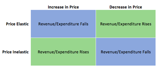
The key concept in thinking about collecting the most revenue is the price elasticity of demand. Total revenue is price times the quantity of tickets sold. Imagine that the band starts off thinking about a certain price, which will result in the sale of a certain quantity of tickets. The three possibilities are in Fig 6.7. If demand is elastic at that price level, then the band should cut the price, because the percentage drop in price will result in an even larger percentage increase in the quantity sold—thus raising total revenue. However, if demand is inelastic at that original quantity level, then the band should raise the ticket price because a certain percentage increase in price will result in a smaller percentage decrease in the quantity sold—and total revenue will rise. If demand has a unitary elasticity at that quantity, then an equal percentage change in quantity will offset a moderate percentage change in the price—so the band will earn the same revenue whether it (moderately) increases or decreases the ticket price.
| If Demand Is . . . | Then . . . | Therefore . . . |
|---|---|---|
| Elastic | % change in Qd > change in P | A given % rise in P will be more than offset by a larger % fall in Q so that total revenue (P × Q) falls. |
| Unitary | % change in Qd = % change in P | A given % rise in P will be exactly offset by an equal % fall in Q so that total revenue (P × Q) is unchanged. |
| Inelastic | % change in Qd < change in P | A given % rise in P will cause a smaller % fall in Q so that total revenue (P × Q) rises. |
Fig 6.6
What if the band keeps cutting price, because demand is elastic until it reaches a level where it sells all 15,000 seats in the available arena? If demand remains elastic at that quantity, the band might try to move to a bigger arena, so that it could slash ticket prices further and see a larger percentage increase in the quantity of tickets sold. However, if the 15,000-seat arena is all that is available or if a larger arena would add substantially to costs, then this option may not work.
Conversely, a few bands are so famous or have such fanatical followings, that demand for tickets may be inelastic right up to the point where the arena is full. These bands can, if they wish, keep raising the ticket price. Ironically, some of the most popular bands could make more revenue by setting prices so high that the arena is not full—but those who buy the tickets would have to pay very high prices.
The table below summarizes the relationship between price and total revenue
What about Expenditure?
You will notice that expenditure is mentioned whenever revenue is. This is because a dollar earned by the band corresponds to a dollar spent by the consumer. Therefore, if the band’s revenue is rising, then the consumer’s expenditure is rising as well. You must understand how to answer questions from both sides.
Can Business Pass Costs on to Consumers?
Imagine that as a consumer of legal pharmaceutical products, you read a newspaper story that a technological breakthrough in the production of aspirin has occurred, so that every aspirin factory can now produce aspirin more cheaply. What does this discovery mean to you? Fig 6.8 A illustrates two possibilities. In Panel A, the demand curve is highly inelastic. In this case, a technological breakthrough that shifts supply to the right, from S0 to S1, so that the equilibrium shifts from E0 to E1, creates a substantially lower price for the product with relatively little impact on the quantity sold. In Panel B, the demand curve is highly elastic. In this case, the technological breakthrough leads to a much greater quantity sold in the market at very close to the original price. Consumers benefit more, in general, when the demand curve is more inelastic because the shift in the supply results in a much lower price for consumers.
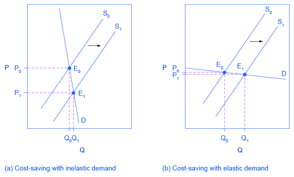
Since demand for food is generally inelastic, farmers may often face the situation in Panel A. That is, a surge in production leads to a severe drop in price that can actually decrease the total revenue that farmers receive. Conversely, poor weather or other conditions that cause a terrible year for farm production can sharply raise prices so that the total revenue that the farmer receives, increases.
Attribution
“4.2 Elasticity and Revenue” in Principles of Microeconomics by Dr. Emma Hutchinson, University of Victoria is licensed under a Creative Commons Attribution 4.0 International License, except where otherwise noted.
“5.3 Elasticity and Pricing” in Principles of Economics 2e by OpenStax is licensed under Creative Commons Attribution 4.0 International License.
