4.4 Taxes and Deadweight Loss
Taxes are not the most popular policy, but they are often necessary. We will look at two methods to understand how taxes affect the market: by shifting the curve and using the wedge method.
When the government sets a tax, it must decide whether to levy the tax on the producers or the consumers. This is called legal tax incidence. The most well-known taxes are ones levied on the consumer, such as Government Sales Tax (GST) and Provincial Sales Tax (PST). The government also sets taxes on producers, such as the gas tax, which cuts into their profits. The legal incidence of the tax is actually irrelevant when determining who is impacted by the tax. When the government levies a gas tax, the producers will pass some of these costs on as an increased price. Likewise, a tax on consumers will ultimately decrease quantity demanded and reduce producer surplus.
When the government imposed a gas tax for example, from the producer’s perspective, any tax levied on them is just an increase in the marginal costs per unit. To illustrate the effect of a tax, let’s look at the oil market again.
Example
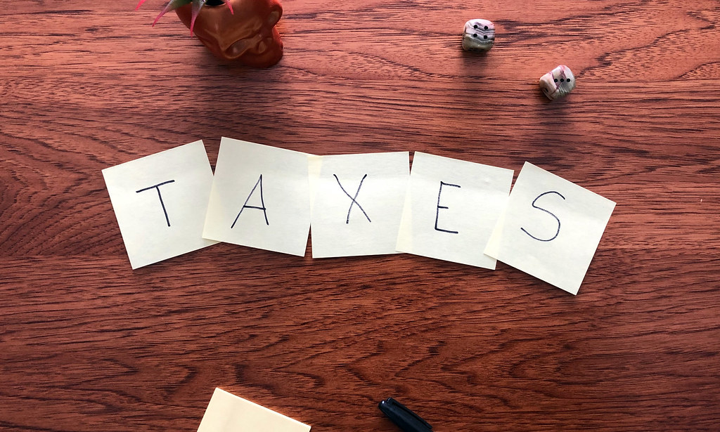
If the government levies a $3 gas tax on producers, the supply curve will shift up by $3. As shown in Fig 4.16 below, a new equilibrium is created at P=$5 and Q=2 million barrels. Note that producers do not receive $5, they now only receive $2, as $3 has to be sent to the government. From the consumer’s perspective, this $1 increase in price is no different than a price increase for any other reason and responds by decreasing the quantity demanded the higher priced good.
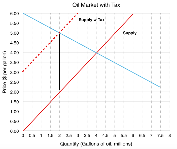
What if the legal incidence of the tax is levied on the consumers? Since the demand curve represents the consumers’ willingness to pay, the demand curve will shift down as a result of the tax, as shown in Fig 4.17 below. If consumers are only willing to pay $4/gallon for 4 million gallons of oil but know they will face a $3/gallon tax, they will only purchase 4 million gallons if the ticket price is $1. This creates a new equilibrium where consumers pay a $2 ticket price, knowing they will have to pay a $3 tax for a total of $5. The producers will receive the $2 paid before taxes.
Tax Wedge
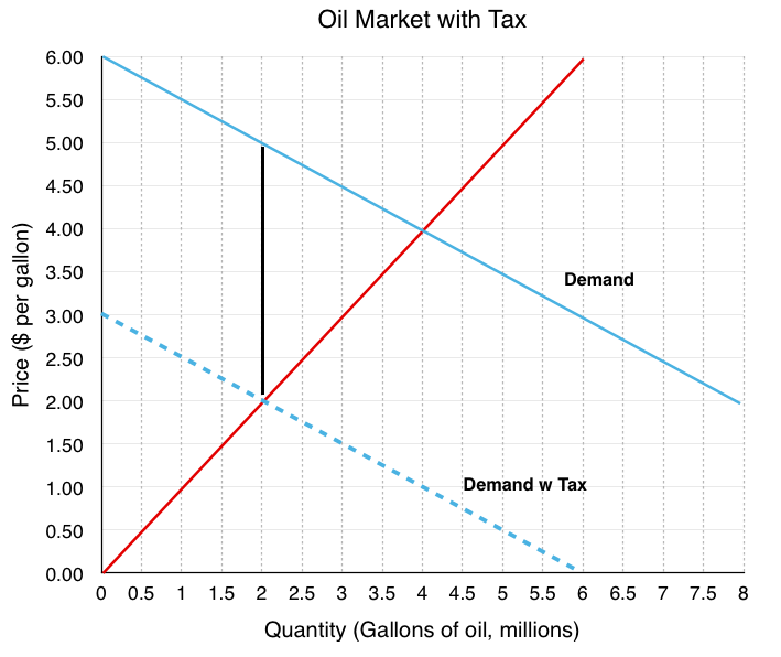
Another method to view taxes is through the wedge method. This method recognizes that who pays the tax is ultimately irrelevant. Instead, the wedge method illustrates that a tax drives a wedge between the price consumers pay and the revenue producers receive, equal to the size of the tax levied.
As illustrated below in Fig 4.18, to find the new equilibrium, one simply needs to find a $3 wedge between the curves. The first wedge tested is only $0.7, followed by $1.5, until the $3.0 tax is found.
Economic Impact of tax
Like with price and quantity controls, one must compare the market surplus before and after a price change to fully understand the effects of a tax policy on surplus. Before the tax is imposed, economic surplus or market surplus is maximized as shown in Fig 4.19 A below.
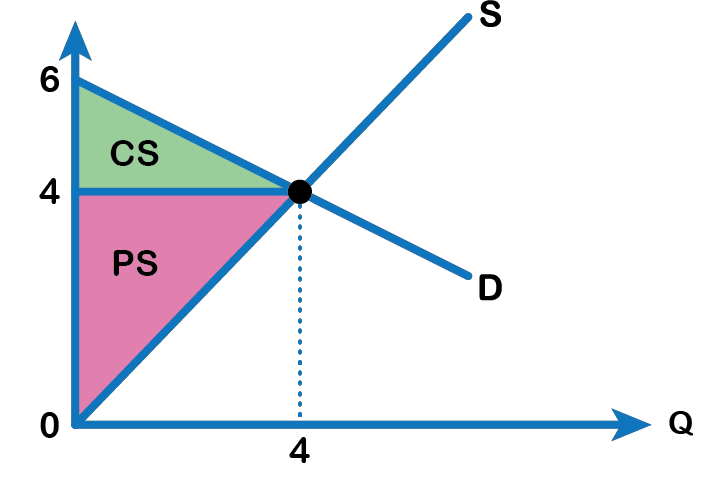
Before
The market surplus before the tax can be calculated from Fig 4.19 A. Ensure you understand how to get the following values:
- Consumer Surplus = $4 million
- Producer Surplus = $8 million
- Market Surplus = $12 million
After
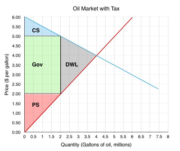
The market surplus after the policy can be calculated in reference to Fig 4.19 B.
- Consumer Surplus (Blue Area) = $1 million
- Producer Surplus (Red Area) = $2 million
- Government Revenue (Green Area) = $6 million
- Market Surplus = $9 million
Transfer and Deadweight Loss
Let’s look closely at the tax’s impact on quantity and price to see how these components affect the market.
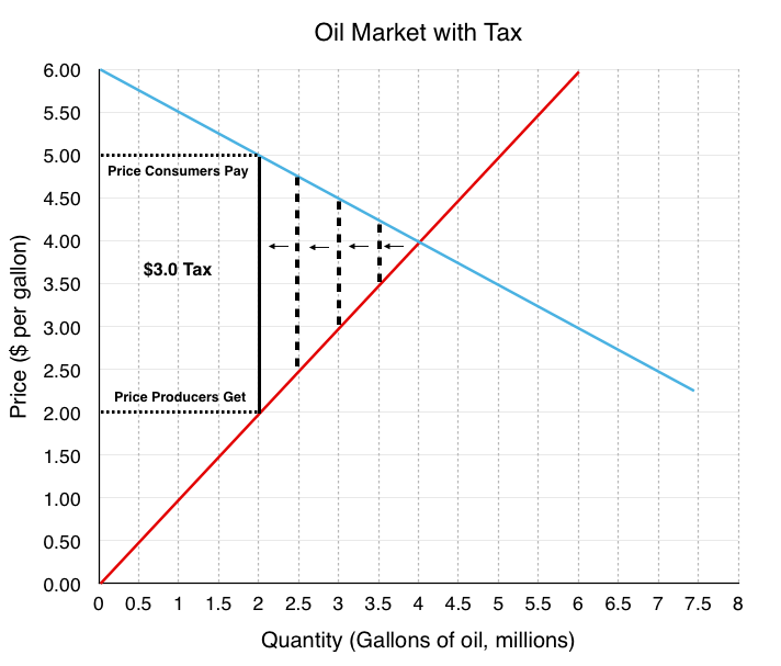
![Areas: A(blue) [(0,5)(2,5)(2,4)(0,4)], B(dark grey) [(2,5)(4,4)(2,4)], C(red) [(0,4)(2,4)(2,2)(0,2)], D(light grey) [(2,4)(4,4)(2,2)]](https://ecampusontario.pressbooks.pub/app/uploads/sites/2340/2022/02/Oil-market-with-tax-5.png)
Transfer – The Impact of Price
Due to the tax’s effect on the price, areas A and C are transferred from consumer and producer surplus to government revenue.
- Consumers to Government – Area A – Consumers originally paid $4/gallon for gas. Now, they are paying $5/gallon. The $1 increase in price is the portion of the tax that consumers have to bear. This price change means the government collects $1 × 2 million gallons or $2 million in tax revenue from the consumers.
- Producers to Government – Area C- Originally, producers received revenue of $4/gallon for gas. Now, they receive $2/gallon. This $2 decrease is the portion of the tax that producers have to bear. This means that the government collects $2 × 2 million gallons or $4 million in tax revenue from the producers. This is a transfer from producers to the government.
Deadweight Loss – The Impact of Quantity
A higher price for consumers will cause a decrease in the quantity demanded, and a lower price for producers will cause a decrease in quantity supplied. This reduction from equilibrium quantity is what causes a deadweight loss in the market since there are consumers and producers who are no longer able to buy and supply the good.
Taxes are more complicated than price control as they involve a third economic player: the government. As we saw, who the tax is levied on, is irrelevant when looking at how the market ends up. Note that the last three sections have painted a fairly grim picture about policy instruments. This is because our model currently does not include the external costs economic players impose on the macro-environment (pollution, disease, etc.). These concepts will be explored in more detail in the next chapter.
Attribution
“4.7 Taxes and Subsidies” in Principles of Microeconomics by Dr. Emma Hutchinson, University of Victoria is licensed under a Creative Commons Attribution 4.0 International License, except where otherwise noted.
