4.3 Inefficiency of Price Floor and Price Ceiling
To this point in the chapter, we have been assuming that markets are free, that is, they operate with no government intervention. In this section, we will explore the outcomes, both anticipated and otherwise, when the government does intervene in a market either to prevent the price of some good or service from rising “too high” or to prevent the price of some good or service from falling “too low”.
In perspective
Economists believe there are a small number of fundamental principles that explain how economic agents respond in different situations. Two of these principles, which we have already introduced, are the laws of demand and supply. Governments can pass laws affecting market outcomes, but no law can negate these economic principles. Rather, the principles will become apparent in sometimes unexpected ways, which may undermine the intent of the government policy. This is one of the major conclusions of this section.
The imposition of or a price ceiling a price floor will prevent a market from adjusting to its equilibrium price and quantity, and thus will create an inefficient outcome. However, there is an additional twist here. Along with creating inefficiency, price floors and ceilings will also transfer some consumer surplus to producers, or some producer surplus to consumers.
Price Ceiling
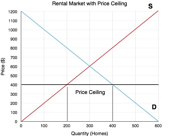
Calculating Market Surplus
To find out the impact of the government’s price ceiling, we must calculate market surplus before, and after a policy. This method will be an important gauge for all our policy analysis on this topic. Consider Fig 4.9 (A & B), where the effects of the Price Ceiling are shown.
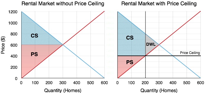
“Rental Market without and with Price Ceiling” by Dr. Emma Hutchinson, University of Victoria, CC BY 4.0.
Before the Ceiling
The calculation of market surplus before policy intervention should be straightforward by now. Market surplus is equal to the sum of consumer surplus and producer surplus, calculated from Fig 4.9 (A):
- Consumer Surplus (Blue Area): [(1200 − 600) × 300] ÷ 2 = $90,000
- Producer Surplus (Red Area): [(600) × 300] ÷ 2 = $90,000
- Total Surplus: $180,000
After the ceiling
The calculation of market surplus after the intervention is less obvious. Consumers have lost surplus in some areas, but gained surplus in others (we will look at this closely in the next Fig 4.10). Producers have lost surplus. From Fig 4.9 (B),
- Consumer Surplus (Blue Area): [(1200 − 800) × 200] ÷ 2] + (400 × 200) = $120,000
- Producer Surplus (Red Area): [(600) × 300] ÷ 2 = $40,000
- Total Surplus: $160,000
The rent ceiling results in a loss in the total surplus to the society.
What about Redistribution?
 It’s easy to look at the total numbers and show that market (total) surplus has decreased, but how does this change affect individual consumers and firms?
In Fig 4.10, the areas which change as a result of the policy, are shown.
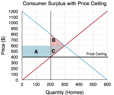
| Consumers | Consumers gain an area of A and lose an area of B.
As mentioned previously, the quantity supplied in the market decreases from 300 rental units to 200 under the price ceiling, and also there is a shortage of 200 homes due to this policy. We can assume that some consumers get the advantage of the price ceiling are benefitted. They are now paying $400 a month instead of the earlier rent of $600 a month for a rental home. This is shown in Fig 4.11 as area A. A price ceiling, as observed from Fig 4.11 above, shows a loss in consumer surplus, identified as area B, and a gain in consumer surplus shown as area A. |
| Producers | Producers lose areas C and A.
The price ceiling causes the landlords to reconsider staying in the rental market, as fewer landlords can make a profit with the lower price. Due to the ceiling, 100 landlords leave the market, thus reducing their producer surplus identified as area B in Fig 4.11. Like consumers, some producers will remain in the market, but these producers now have to face the reality of lower rent revenue and therefore they lose area A. This area which used to be a part of producer surplus, prior to the rent ceiling, is now transferred to the consumers or renters. |
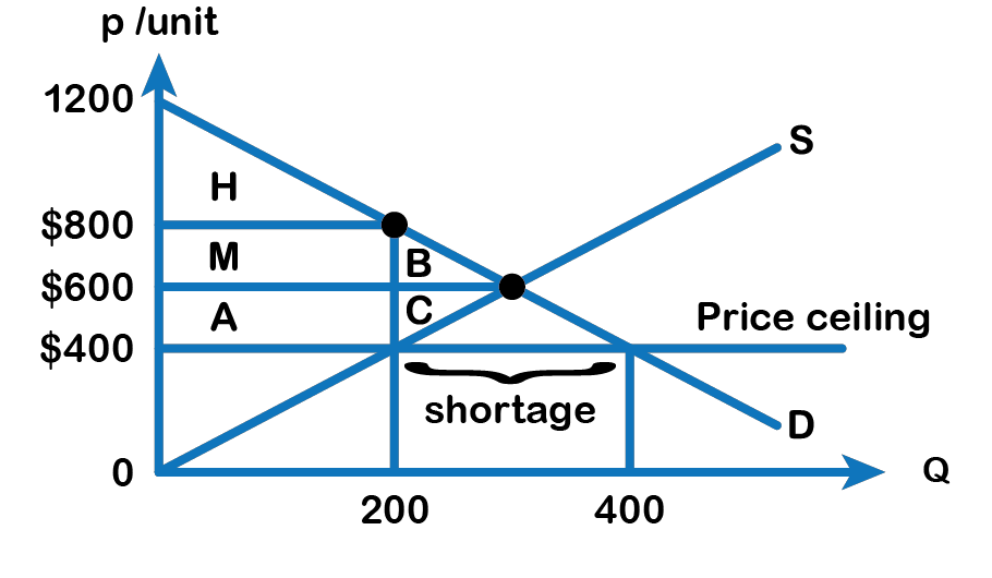
| Black Market due to Rent Ceiling | However, the shortage increases the difficulty of finding a rental unit. This could result in some consumers willing to pay most for the homes, a rent as high as $800, to ensure the availability of a rental unit, therefore violating government’s price ceiling. This is a black market transaction.
If the tenants engage in black market activity by paying a rent of $800, then consumer surplus shrinks to area H. The areas M + A get transferred from renters (consumers) to producers (landlords), as shown in Fig 4:11. |
| Deadweight Loss | The deadweight loss or a loss in total surplus to the society due to a price ceiling arises because there are players who are no longer able to be a part of the market. 100 renters and 100 landlords all lose a varied amount based on their willingness to pay and marginal cost.
This was a fairly lengthy explanation of price ceilings, but it is one that will lead to the discussion of all policies. Every policy we will look at in microeconomics has both a quantity effect and a price effect, and it is important to understand how the policy impacts individual market players. Some people gain while some people lose as a result of this government policy. Therefore, we can infer price ceiling has a mixed effect and there is a loss of economic efficiency which is represented by areas B + C. |
Price Floor in the Labour Market (Minimum Wage Law)
While the price floor has a very similar analysis to the price ceiling, it is important to look at it separately. A common example of a price floor is a minimum wage policy. The labour market is unique in that the workers are the producers of labour and the firms are consumers of labour. Price can be denominated in hourly wage, with the quantity of workers on the x-axis. If the government sets a binding minimum wage (price floor), it must be set above the equilibrium price.
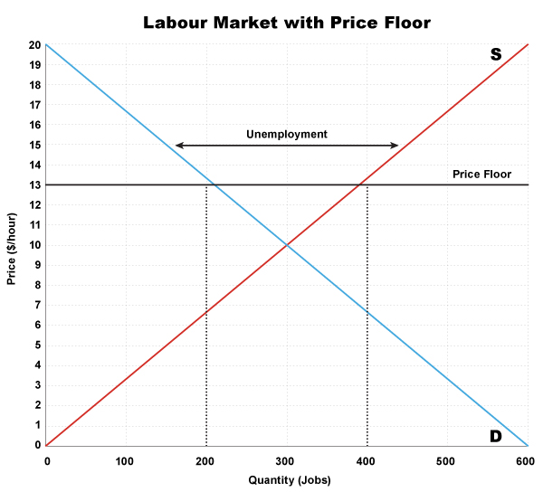
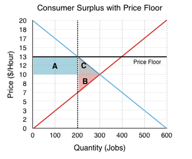
In Fig 4.12, the equilibrium wage is shown as $10/hour. This is where the demand for labour is equal to the number of workers who want to find jobs. At this level there is no unemployment. However, if the government sets a minimum wage of $13/hour, this will change. The Quantity of Labour Supplied (workers looking for jobs) will be 400, but the quantity demanded will be 200. This means that 200 workers will be unemployed! Again, this is not enough information to determine whether the market is inefficient – we have to calculate the change in total surplus!
“Labour Market without and with Price Floors“, by Dr. Emma Hutchinson, University of Victoria, CC BY 4.0
Using the same process as before:
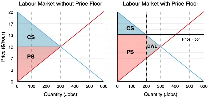
Before (from Fig 4.13 A)
- Consumer Surplus (Blue Area): [(20 − 10) × 300] ÷ 2 = $1500
- Producer Surplus (Red Area): [(10) × 300] ÷ 2 = $1500
- Total (Market) Surplus: $3000
After (from Fig 4.13 B)
- Consumer Surplus (Blue Area): [(20 − 13) × 200] ÷ 2= $700
- Producer Surplus (Red Area): [(13 − 7) × 200] + (7 × 200) ÷ 2 = $1900
- Total Surplus: $2600
Since the total surplus after the policy is less than the total surplus before, there is a deadweight loss!
Again, the changes in the market can be categorized as a transfer and a deadweight loss. This time, the transfer is from consumers (firms) to producers (workers), since the workers who are able to find work are better off. This causes no change to market surplus in isolation but is coupled with the deadweight loss caused by workers who are no longer able to find jobs as firms leave the market. The deadweight loss is represented by areas B + C.
Price Floor in the Market for Movie Theatres

Fig 4.15 shows a price floor example using a string of struggling movie theatres, all in the same city. The current equilibrium is $8 per movie ticket, with 1,800 people attending movies. The original consumer surplus is A + B + D, and original the producer surplus is C + E. The city government is worried that movie theatres will go out of business, reducing the entertainment options available to citizens, so it decides to impose a price floor of $12 per ticket. As a result, the quantity demanded of movie tickets falls to 1,400. The new consumer surplus is A, and the new producer surplus is C + B. In effect, the price floor causes area B to be transferred from consumers to producers but also causes a deadweight loss of D + E.
In the next section, we will see the economic impact of a tax policy, which also results in a deadweight loss.
Attributions
“4.5 Price Controls” in Principles of Microeconomics by Dr. Emma Hutchinson, University of Victoria is licensed under a Creative Commons Attribution 4.0 International License, except where otherwise noted.
“3.5 Demand, Supply, and Efficiency” in Principles of Economics 2e by OpenStax is licensed under Creative Commons Attribution 4.0 International License.
