6.1 Price Elasticity of Demand
Anyone who has studied economics knows the law of demand: a higher price will lead to a lower quantity demanded. What you may not know is how much lower the quantity demanded will be. This topic will explain how to answer these questions and why they are critically important in the real world.
Definition: Price Elasticity of Demand
Elasticity is an economics concept that measures the responsiveness of one variable to changes in another variable. The price elasticity of demand is the percentage change in the quantity demanded of a good or service divided by the percentage change in the price. This shows the responsiveness of the quantity demanded to a change in price. Because price and quantity demanded move in opposite directions, the price elasticity of demand is always a negative number. Therefore, price elasticity of demand is usually reported as an absolute value, without a negative sign.
Price Elasticity of Demand = % change in Quantity demanded ÷ % change in Price
Example
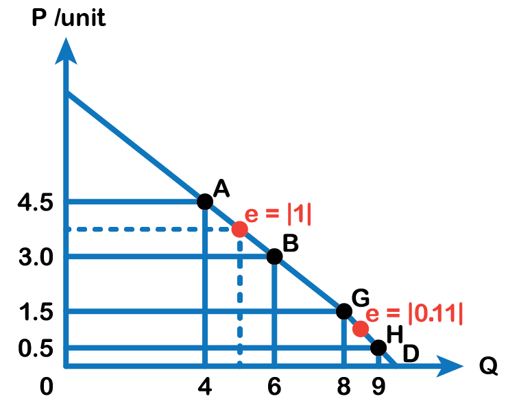
Look at the above figure. When the price of a cup of coffee is $4.5, the quantity demanded is 4 cups an hour and when the price falls to $3.00 a cup, the quantity demanded rises to 6 cups every hour.
Moving from Point A to B:
- % Change in Price: The coffee price falls from $4.50 to $3.00, meaning the percentage change is [(3.00 − 4.50) ÷ 4.50] × 100 = −33%. Price has fallen by 33%
- % Change in Quantity Demanded: The quantity of coffee sold increases from 4 to 6, meaning the percentage change is [(6 − 4) ÷ 4] × 100 = 50%. The quantity has risen by 50%
Therefore, Elasticity: %change in Quantity demanded ÷ %change in Price = −50% ÷ 33% = −1.5.
In absolute terms, elasticity = 1.5. This is the price elasticity of demand over the range of the demand curve between points A and B.
Midpoint Method
To calculate elasticity, instead of using simple percentage changes in quantity and price, economists use the average percent change. This is called the mid-point method for elasticity, and is represented in the following equations:
% change in quantity demanded = [(New Q − Old Q) ÷ ((New Q + Old Q) ÷ 2)] × 100%
- (New Q + Old Q) ÷ 2 shows the average of the two quantities
% change in price = [(New Price − Old Price) ÷ ((New P + Old P) ÷ 2)] × 100%
- (New P +Old P) ÷ 2 is the average of the two prices
The advantage of the mid-point method is that we find the elasticity right at a single point on the demand curve, which is more precise than finding the elasticity over the entire range between the two points A and B, in the above figure.
Using the mid-point method to calculate the elasticity between Point A and Point B:
This method gives us a sort of average elasticity of demand at the centre point between the two points on our demand curve. The elasticity of demand is interpreted as when the price changes by 1 percent, the quantity demanded also changes by 1 percent.
Is Elasticity the Slope?
It is a common mistake to confuse the slope of the demand curve with its elasticity. The slope is the rate of change in units along the curve, or the rise/run (change in y over the change in x).
Example
In Fig 6.1, at each point between A and B, shown on the demand curve, price drops by $1.50 and the number of units demanded increases by 2. The slope is –1.5/2 = – 0.75 along the entire demand curve and does not change. The price elasticity, however, changes along the curve. The elasticity between points A and B was – 1 and changed to – 0.11 between points G and H. Elasticity is the percentage change, which is a different calculation from the slope and has a different meaning.
Different Kinds of Price Elasticities of Demand
We can usefully divide elasticities into three broad categories: elastic, inelastic, and unitary.
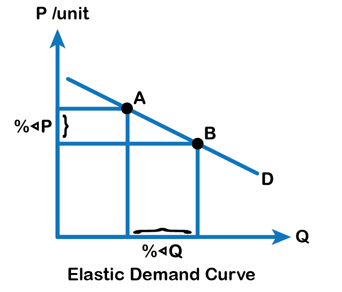
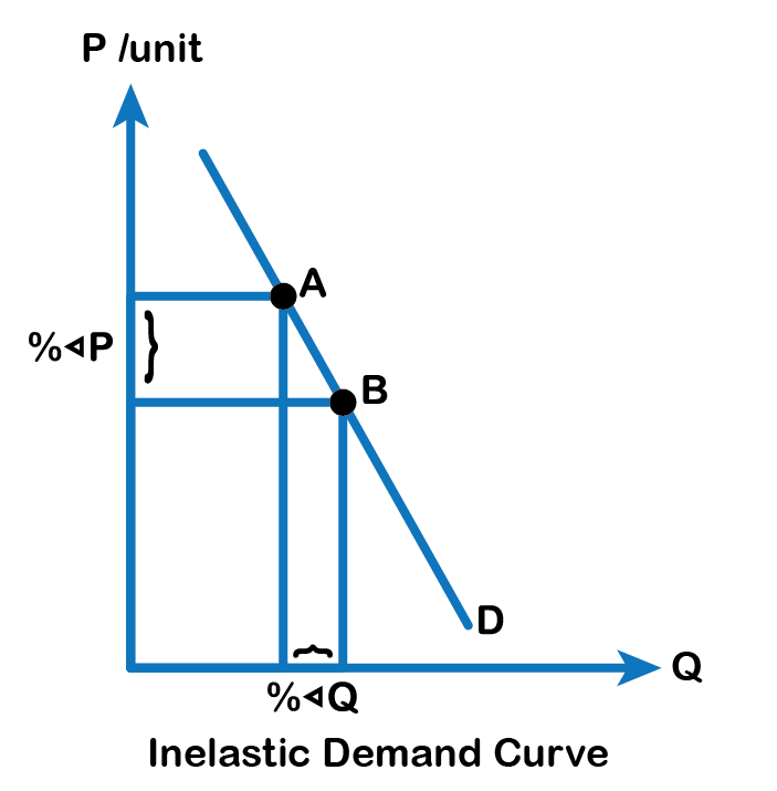
Elastic demand is one in which the elasticity is greater than one, indicating high responsiveness to changes in price (Fig 6.2 A). Elasticities that are less than one indicate low responsiveness to price changes and correspond to inelastic demand (Fig 6.2 B). An elastic demand curve is relatively flatter than an inelastic demand curve. Unitary elastic demand indicates quantity demanded changes by the same proportion with respect to the price, as Fig 6.3 below summarizes.
| If... | Then... | And it is called... |
|---|---|---|
| % change in quantity > % change in price | % change in quantity ÷ % change in price > 1 | Elastic |
| % change in quantity = % change in price | % change in quantity ÷ % change in price = 1 | Unitary |
| % change in quantity < change in price | % change in quantity ÷ % change in price < 1 | Inelastic |
Fig 6.3
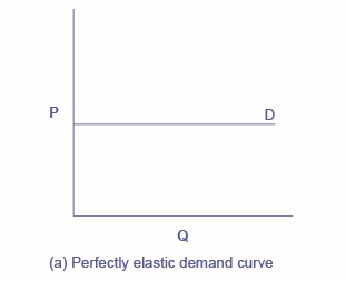
There are two extreme cases of elasticity: when elasticity equals zero and when it is infinite. We will describe each case. Infinite elasticity or perfect elasticity refers to the extreme case where the quantity demanded changes by an infinite amount in response to any change in price at all. In this case, the demand curve is horizontal as Fig 6.4 A shows. Perfectly elastic demand is an extreme example. Examples of such goods are Caribbean cruises and sports vehicles.
Zero elasticity or perfect inelasticity, as Fig 6.4 B depicts, refers to the extreme case in which a percentage change in price, no matter how large, results in zero change in quantity. Again, while perfectly inelastic demand is an extreme case, necessities are likely to have highly inelastic demand curves. This is the case with life-saving drugs and gasoline.
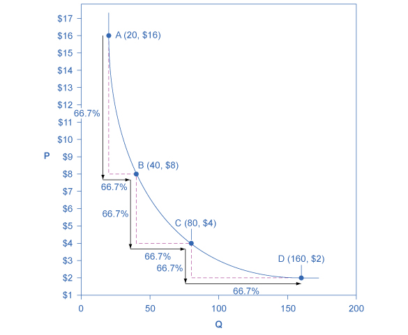
Constant unitary elasticity, in a demand curve, occurs when a price change of one percent results in a quantity change of one percent. Fig 6.4 C shows a demand curve with constant unit elasticity. Using the midpoint method, you can calculate that between points A and B on the demand curve, the price changes by 66.7%, and quantity demanded also changes by 66.7%. Hence, the elasticity equals 1. Between points B and C, price again changes by 66.7% as does quantity, while between points C and D the corresponding percentage changes are again 66.7% for both price and quantity. In each case, then, the percentage change in price equals the percentage change in quantity, and consequently, elasticity equals 1.
Attribution
“4.1 Calculating Elasticity” in Principles of Microeconomics by Dr. Emma Hutchinson, University of Victoria is licensed under a Creative Commons Attribution 4.0 International License, except where otherwise noted.
“5.1 Price Elasticity of Demand and Elasticity of Supply” and “5.2 Polar Cases of Elasticity and Constant Elasticity” in Principles of Economics 2e by OpenStax is licensed under Creative Commons Attribution 4.0 International License.
