7.5 Long Run Costs: The Advantage of Flexibility

Short-run average costs are constrained by the presence of a fixed input. So in the long run we can always do at least as well as, and often better than, in the short run with respect to cost. We can see this is true by comparing the long-run and short-run average cost curves.
Shapes of Long-Run Average Cost Curves
While in the short run firms are limited to operating on a single average cost curve (corresponding to the level of fixed costs they have chosen), in the long run when all costs are variable, they can choose to operate on any average cost curve. Thus, the long-run average cost (LRAC) curve is actually based on a group of short-run average cost (SRAC) curves, each of which represents one specific level of fixed costs. More precisely, the long-run average cost curve will be the least expensive average cost for producing any level of output. Fig 7.9 shows how we build the long-run average cost curve from a group of short-run average cost curves. Five short-run-average cost curves appear on the diagram. Each SRAC curve represents a different level of fixed costs.
Example
Imagine SRAC1 as a small factory, SRAC2 as a medium factory, SRAC3 as a large factory, and SRAC4 and SRAC5 as very large and ultra-large. Although this diagram shows only five SRAC curves, presumably there are an infinite number of other SRAC curves between the ones that we show. Think of this family of short-run average cost curves as representing different choices for a firm that is planning its level of investment in fixed cost physical capital—knowing that different choices about capital investment in the present will cause it to end up with different short-run average cost curves in the future.
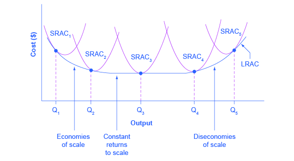
The long-run average cost curve shows the cost of producing each quantity in the long run when the firm can choose its level of fixed costs and thus choose which short-run average costs it desires. If the firm plans to produce in the long run at an output of Q3, it should make the set of investments that will lead it to locate on SRAC3, which allows producing q3 at the lowest cost. A firm that intends to produce Q3 would be foolish to choose the level of fixed costs at SRAC2 or SRAC4. At SRAC2 the level of fixed costs is too low for producing Q3 at the lowest possible cost, and producing q3 would require adding a very high level of variable costs and make the average cost very high. At SRAC4, the level of fixed costs is too high for producing q3 at the lowest possible cost, and again average costs would be very high as a result.
The shape of the long-run cost curve, in Fig 7.10, is fairly common for many industries. The left-hand portion of the long-run average cost curve, where it is downward-sloping from output levels Q1 to Q2 to Q3, illustrates the case of economies of scale. In this portion of the long-run average cost curve, a larger scale leads to lower average costs.
The right-hand portion of the long-run average cost curve, running from output level Q4 to Q5, shows a situation where, as the level of output and the scale rises, average costs rise as well. A firm or a factory can grow so large that it becomes very difficult to manage, resulting in unnecessarily high costs as many layers of management try to communicate with workers and with each other, and as failures to communicate lead to disruptions in the flow of work and materials.
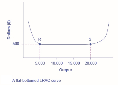
In the middle portion of the long-run average cost curve, the flat portion of the curve around Q3, economies of scale have been exhausted. In this situation, allowing all inputs to expand does not much change the average cost of production.
In this LRAC curve range, the average cost of production does not change much as scale rises or falls.
Economies and Diseconomies of Scale
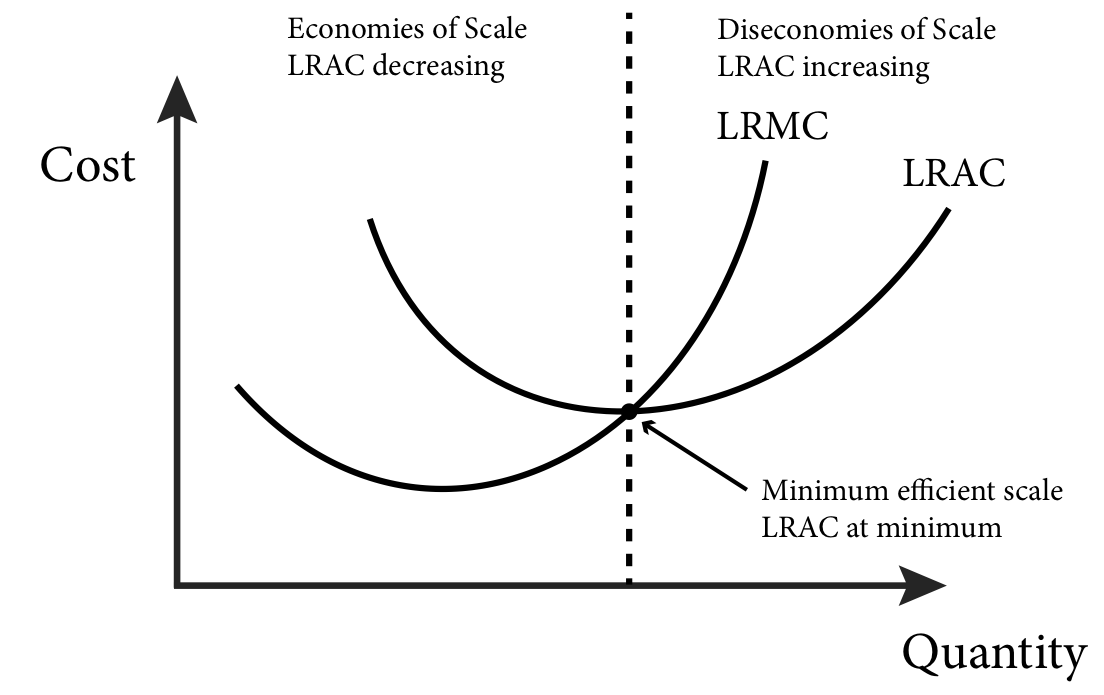
An important economic concept associated with the long-run average cost curve is economies of scale. Economies of scale occur when the average cost of production falls as output increases. Economies of scale refer to the situation where, as the quantity of output goes up, the cost per unit goes down. This is the idea behind “warehouse stores” like Costco or Walmart. In everyday language: a larger factory can produce at a lower average cost than a smaller factory. Similarly, diseconomies of scale occur when the average cost of production rises as output increases. Constant returns to scale (Fig 7.11) occur when the average cost of production does not change as output rises. In a typical long-run average cost curve, there are sections of both economies of scale and diseconomies of scale. There is also a point or region of minimum efficient scale where the average cost is at its minimum. This is the point where economies of scale are used up and no longer benefit the firm. Figure 7.12 illustrates these points.
Attribution
“7.5 Costs in the Long Run” in Principles of Economics 2e by OpenStax is licensed under Creative Commons Attribution 4.0 International License.
“Module 8: Cost Curves” in Intermediate Microeconomics by Patrick M. Emerson is licensed under a Creative Commons Attribution-NonCommercial-ShareAlike 4.0 International License, except where otherwise noted.
