9.2 Single Price Monopoly Demand and Marginal Revenue
So we know a competitive market faces an elastic demand, what about a single-priced monopoly? This is distinct from other monopolies in that the firm must charge the same price to all consumers. In this case, the aggregate demand is the firm’s demand!
Example: The Sunglass Market
To explore monopoly, consider the sunglasses market. What do Oakley, Ray-Ban and Persol have in common? They are all owned by the same brand. That’s right, Luxottica, an Italian-based eyewear company, produces about 70% of all name-brand eyewear. This is fairly close to a monopoly, as with that high of a market share, Luxottica dominates the market price. Notice that Luxottica is not a single price monopoly, as it practices a form of price discrimination by having multiple brands aimed at different consumers.
Let’s consider what would happen if Luxottica only sold one kind of sunglasses at the same price to all consumers, and if they owned 100% of the market. Whereas the competitive firm was a small player in the aggregate market, the monopolist dictates both the final price and the quantity. If Luxottica decides to lower the price, it must do so for ALL buyers. Consider what implications this has on revenue.
According to the law of demand, as price falls, the quantity demanded increases. This means that Luxottica can increase revenue by lowering prices, as they sell more sunglasses. This is not what happens from a price decrease however, as the firm decreases its price it loses some of the revenue on the goods it was previously selling.
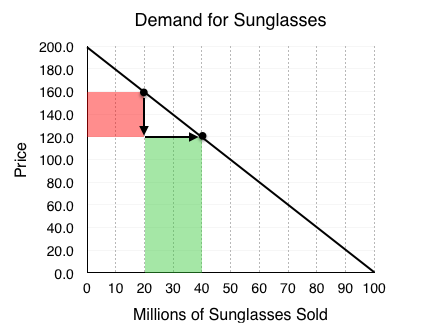
As shown in Fig 9.2, Luxottica is selling 20 million sunglasses at $160 per pair. When it reduces the price to $120, two things happen:
- Luxottica loses $40 on each of the 20 million sunglasses it was selling before. 20 million consumers were willing to pay the full $160 for a pair, and now only have to pay $120. This results in a loss of $800 million for Luxottica. (shown as the red shaded region in Fig 9.2).
- Luxottica gains $120 on each of the 20 million new sunglasses it now sells. 20 million consumers were not willing to pay $160 for a pair, but are willing to pay $120. This results in a gain of $2.4 billion for Luxottica (shown as the green shaded region in Fig 9.2).
These changes collectively represent a net gain of $1.6 billion for Luxottica. This net gain is the marginal revenue earned by Luxottica (Total revenue of $120b × 40 – $160b × 20 = $1.6 billion).
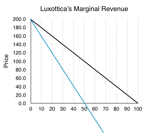
For a single-price monopolist, marginal revenue is less than the price at each quantity of output (P > MR). Therefore, the marginal revenue curve lies below the demand curve for a monopolist.
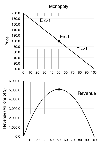
Remember, the equation to calculate the elasticity of demand ED is (% change in quantity ÷ % change in price). Looking at the change in revenue from the examples above, we can see that the decrease in revenue came from the price change, and the increase came from the quantity change. This means that when % change in quantity > % change in price, our revenue increases from a price drop! Put simply, when our ED>1, we should continue to decrease price, maximizing our revenue. Therefore, the monopolist should operate on the elastic portion of the demand curve.
Competition vs Monopoly
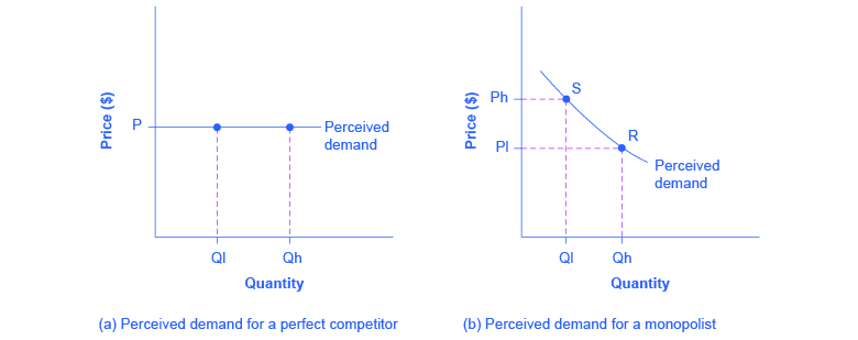
A perfectly competitive firm acts as a price taker and faces a perfectly elastic or horizontal demand curve as shown in Fig 9.5 A. The monopolist is a price maker and faces a downward-sloping demand curve as shown in Fig 9.5 B. As the price is lowered, the quantity demanded increases.
Attribution
“8.1 Monopoly” in Principles of Microeconomics by Dr. Emma Hutchinson, University of Victoria is licensed under a Creative Commons Attribution 4.0 International License, except where otherwise noted.
“9.2 How a Profit-Maximizing Monopoly Chooses Output and Price” in Principles of Economics 2e by OpenStax is licensed under Creative Commons Attribution 4.0 International License.
