5.1 Externalities
To this point, we have modelled private markets. Private markets only consider consumers, producers, and the government – the impacts on external parties are irrelevant. The perfectly competitive market in Chapters 3 and 4 we modelled, offered an efficient way to put buyers and sellers together and determine what goods are produced, how they are produced, and who gets them. The principle that voluntary exchange benefits both buyers and sellers is a fundamental building block of the economic way of thinking. But what happens when a voluntary exchange affects a third party who is neither the buyer nor the seller?
Example
Consider an example of a concert producer who wants to build an outdoor arena that will host country music concerts a half-mile from your neighbourhood. You will be able to hear these outdoor concerts while sitting on your back porch—or perhaps even in your dining room. In this case, the sellers and buyers of concert tickets may both be quite satisfied with their voluntary exchange, but you have no voice in their market transaction. The effect of market exchange on a third party who is outside or “external” to the exchange is called an externality. Because externalities that occur in market transactions affect other parties beyond those involved, they are sometimes called spillovers.
Externalities can be negative or positive. If you hate country music, then having it waft into your house every night would be a negative externality. If you love country music, then what amounts to a series of free concerts would be a positive externality.
Enriching Our Model
As discussed earlier, we have previously modelled private markets. Thus, the terminology we used in that analysis applies to private markets. The terms consumer surplus, producer surplus, market surplus, and the market equilibrium (note that this will be referred to interchangeably in this chapter as the unregulated market equilibrium) derive their meaning from an analysis of private markets and need to be adapted in a discussion where external costs or external benefits are present.
For the purpose of this analysis, the following terminology will be used:
- Our chapter three demand curve is equivalent to the marginal private benefit curve or D.
- Our chapter three supply curve is equivalent to the marginal private cost curve or S.
We now want to develop a model that accounts for positive and negative externalities. To do so, we must consider the external costs and benefits. External costs and benefits occur when producing or consuming a good or service impose a cost/benefit upon a third party.
When we account for external costs and benefits, the following definitions apply:
- When we add external benefits to private benefits, we create a marginal social benefit curve or D-social. In the presence of a positive externality (with a constant marginal external benefit), this curve lies above the demand curve at all quantities.
- When we add external costs to private costs, we create a marginal social cost curve or S-social. In the presence of a negative externality (with a constant marginal external cost), this curve lies above the supply curve at all quantities.
When we were considering private markets, our objective was to maximize market surplus or total private benefits minus total private costs. Our new objective considering all impacted agents in society is to maximize social surplus or total social benefits minus total social costs.
A Negative Externality: Pollution

Pollution is a negative externality. Economists illustrate the social costs of production with a demand and supply diagram. The social costs include the private costs of production that a company incurs and the external costs of pollution that pass on to society.
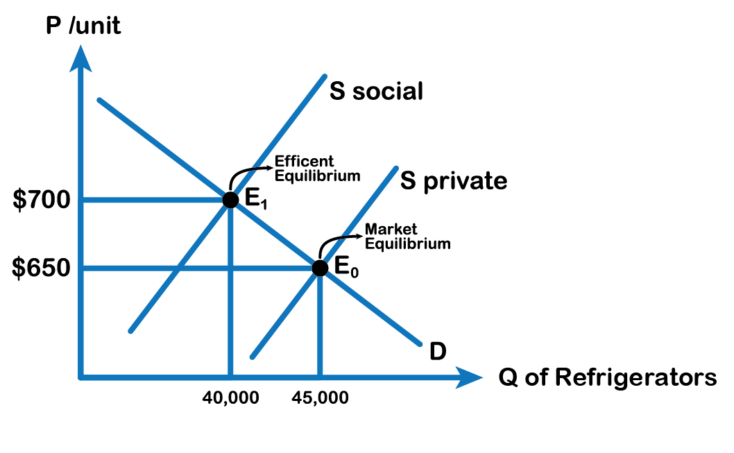
Fig 5.1 shows the demand and supply for manufacturing refrigerators. The demand curve (D) shows the quantity demanded at each price. The supply curve (S) shows the quantity of refrigerators that all firms in the industry supply at each price assuming they are taking only their private costs into account and they are allowed to emit pollution at zero cost. The market equilibrium (E0), where quantity supplied equals quantity demanded, is at a price of $650 per refrigerator and a quantity of 45,000 refrigerators.
However, as a by-product of the metals, plastics, chemicals, and energy that refrigerator manufacturers use, some pollution is created. Let’s say that, if these pollutants were emitted into the air and water, they would create costs of $100 per refrigerator produced. These costs might occur because of adverse effects on human health, or because of other negative impacts. In a market with no anti-pollution restrictions, firms can dispose of certain wastes absolutely free.
In perspective
Now imagine that firms that produce refrigerators must factor in these external costs of pollution—that is, the firms have to consider not only labour and material costs but also the broader costs to society of harm to health and other costs caused by pollution. If the firm is required to pay $100 for the additional external costs of pollution each time it produces a refrigerator, production becomes more costly and the entire supply curve shifts up by $100.
As the Fig. 5.1 above illustrates, the firm will need to receive a price of $700 per refrigerator and produce a quantity of 40,000—and the firm’s new supply curve will be S-social (S plus external costs). The new efficient equilibrium will occur at E1. In short, taking the additional external costs of pollution into account results in a higher price, a lower quantity of production, and a lower quantity of pollution.
If no externalities existed, private costs would be the same as the costs to society as a whole, and private benefits would be the same as the benefits to society as a whole. Thus, if no externalities existed, the interaction of demand and supply will coordinate social costs and benefits. However, when the externality of pollution exists, the supply curve no longer represents all social costs. Because externalities represent a case where markets no longer consider all social costs, but only some of them, economists commonly refer to externalities as an example of market failure. When there is market failure, the private market fails to achieve efficient output, because firms do not account for all costs incurred in the production of output. In the case of pollution, at the market output, social costs of production exceed social benefits to consumers, and the market produces too much of the product.
We can see a general lesson here. If firms were required to pay the social costs of pollution, they would create less pollution but produce less of the product and charge a higher price. In the next section, we will explore the economic impact of positive externalities.
A Positive Externality: Flu Shot

A positive externality occurs when the market interaction of others presents a benefit to non-market participants. The analysis of positive externalities is almost identical to negative externalities. The difference is that instead of the market equilibrium quantity is too much, the market will generate too little Q. Let’s look at an example. Consider the following diagram of a market where a positive externality is present. When someone takes the flu shot, the person not only reduces her own risk of getting the flu but also reduces the chance of people around her contracting the flu. Economists illustrate the social benefits of production with a demand and supply diagram. The social benefits include the private benefits that an individual incurs from the flu shot plus the external benefits of the vaccine that pass on to the community around him.
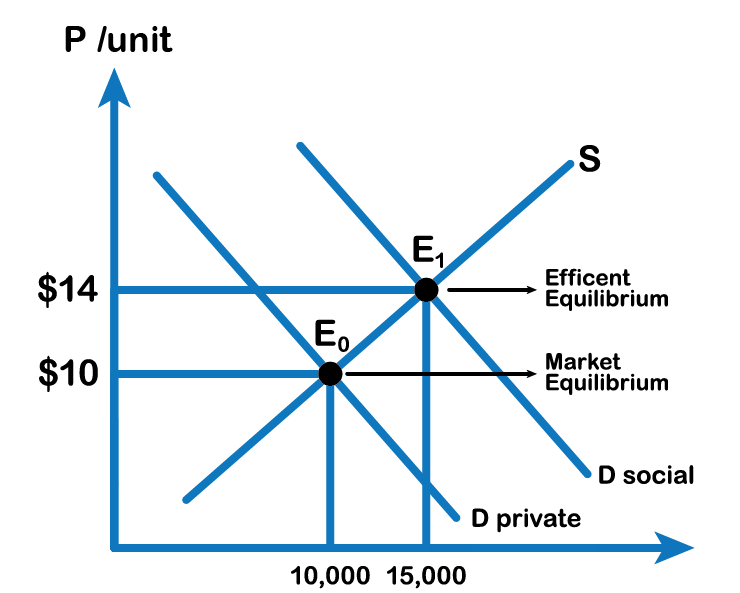
Fig 5.2 shows the demand and supply of Flu shots. The demand curve (D) shows the quantity demanded at each price, taking only the private benefit of receiving the vaccine. The supply curve (S) shows the quantity of flu shots supplied at each price by the pharma industry. The market equilibrium (E0), where quantity supplied equals quantity demanded, is at a price of $10 per shot and a quantity of 10,000 flu shots.
As the Fig 5.2 above shows, the new efficient equilibrium will occur at E1. This is the efficient equilibrium. In short, taking the additional external benefit of the flu shot into account results in a higher price of $14 per shot, and a greater quantity of production (15,000 vaccines). In the case of a positive externality, at the market output, social benefits to consumers are less than the social cost of production, and the market produces too little of the product.
Attribution
“5.1 Externalities” in Principles of Microeconomics by Dr. Emma Hutchinson, University of Victoria is licensed under a Creative Commons Attribution 4.0 International License, except where otherwise noted.
“Chapter 12 Environmental Protection and Negative Externalities” in Principles of Economics 2e by OpenStax is licensed under Creative Commons Attribution 4.0 International License.
