7.2 Theory of Production

Production is the process (or processes) a firm uses to transform inputs (e.g. labour, capital, raw materials) into outputs, i.e. the goods or services the firm wishes to sell.
In perspective

Consider pizza making. The pizzaiolo (pizza maker) takes flour, water, and yeast to make dough. Similarly, the pizzaiolo may take tomatoes, spices, and water to make pizza sauce. The cook rolls out the dough, brushes on the pizza sauce, and adds cheese and other toppings. The pizzaiolo uses a peel—the shovel-like wooden tool—to put the pizza into the oven to cook. Once baked, the pizza goes into a box (if it’s for takeout) and the customer pays for the goods.
We can summarize the ideas so far in terms of a production function, a mathematical expression or equation that explains the engineering relationship between inputs and outputs.
Q = f [L, K]
The production function gives the answer to the question, how much output can the firm produce given different amounts of inputs. We can describe inputs as either fixed or variable.
Definition: Fixed Inputs and Variable Inputs
Fixed inputs are those that can’t easily be increased or decreased in a short period of time. In the pizza example, the building is a fixed input. Once the entrepreneur signs the lease, he or she is stuck in the building until the lease expires. Fixed inputs define the firm’s maximum output capacity.
Variable inputs are those that can easily be increased or decreased in a short period of time. The pizzaiolo can order more ingredients with a phone call, so ingredients would be variable inputs. The owner could hire a new person to work the counter pretty quickly as well. So labor is a variable input.
Economists also differentiate between short and long-run production.
The short-run is the period of time during which at least one or more factors of production are fixed. During the period of the restaurant lease, the pizza restaurant is operating in the short run, because it is limited to using the current building (an example of capital) —the owner can’t choose a larger or smaller building. Plant size or capital is a fixed factor of production in the short run.
The long run is the period of time during which all factors are variable. Once the lease expires for the restaurant, the shop owner can move to a larger or smaller place.
Example
Let’s explore production in the short run using a specific example: offering haircuts in a salon.
Since capital (the salon space) is fixed, the amount of output (e.g. haircuts per day) depends only on the amount of labour employed (e.g. number of barbers working). We can express this production function numerically as the table in Fig 7.1 below shows.
| Number of barbers | Number of haircuts/day |
|---|---|
| 1 | 15 |
| 2 | 22 |
| 3 | 25 |
| 4 | 23 |
| 5 | 19 |
Fig 7.1
Total Product, Marginal Product, and Average Product of Labour
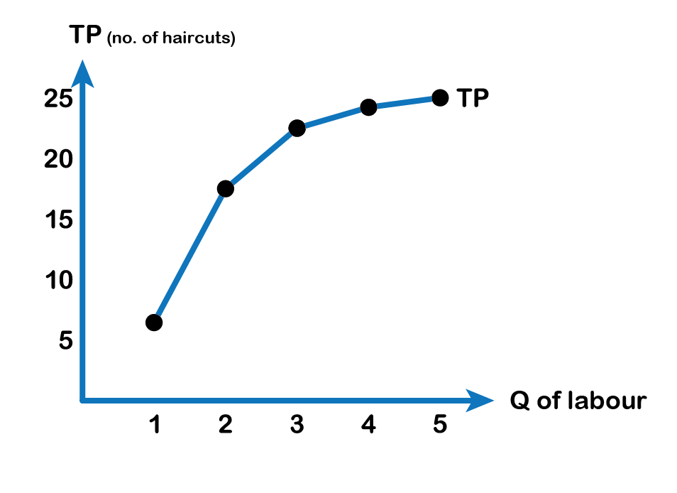
Note that we have introduced some new languages in the above example. We also call Output (Q) as Total Product (TP). TP is the amount of output produced with a given amount of labour and a fixed amount of capital. In this example, one barber can give 15 haircuts in a day. Two barbers can produce 22 haircuts in a day and so on.
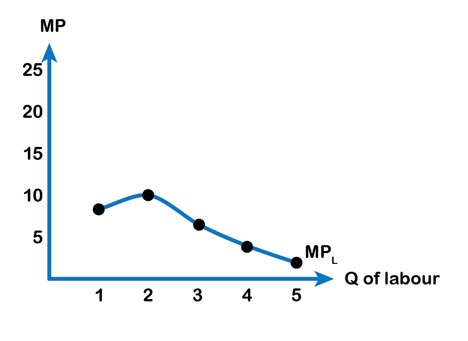
We should also introduce a critical concept: Marginal Product. Marginal product is the additional output of one more worker. Mathematically, Marginal Product is the change in total product divided by the change in labour: MP = ΔTP ÷ ΔL. In the table below (Fig 7.2), since 0 workers produce 0 trees, the marginal product of the first worker is eight haircuts per day, but the marginal product of the second worker is nine haircuts per day.
Short Run production
| Number of barbers | Number of haircuts per day (TP | Marginal Product of labor (MPL) | Average Product of Labor (APL) |
|---|---|---|---|
| 0 | 0 | - | 0 |
| 1 | 8 | 8 | 8 |
| 2 | 17 | 9 | 8.5 |
| 3 | 23 | 6 | 7.6 |
| 4 | 26 | 3 | 6.5 |
| 5 | 27 | 1 | 5.4 |
Fig 7.2
Why might the MPL be rising? To understand the reason behind this pattern, consider that a one-man barbershop is a very busy operation. The single barber needs to do everything: say hello to people, answer the phone, cut hair, clean up, and run the cash register. A second barber reduces the level of disruption from jumping back and forth between these tasks and allows a greater division of labour and specialization. The result can be greater increasing marginal returns. Suppose we add a third barber to the story. What will that person’s marginal product be? What will that person contribute to the salon? However, as other barbers are added, the advantage of each additional barber is less, since the specialization of labour can only go so far. The addition of a third or fourth or fifth barber will have less impact than the second one had. Given the fixed space inside the salon, as additional barbers are hired, they begin bumping elbows and getting in each other’s way. In this case, the addition of still more barbers would cause the output by each worker to decrease and result in falling marginal returns This is called the Law of Diminishing Marginal Product and it’s a characteristic of production in the short run. Why does diminishing marginal productivity occur? It’s because of fixed capital. If the salon manager is unable to lease a larger space but keeps hiring additional barbers, the rate at which TP rises starts to go down and MP decreases.
Below we see how the TP and the MP curves look graphically.


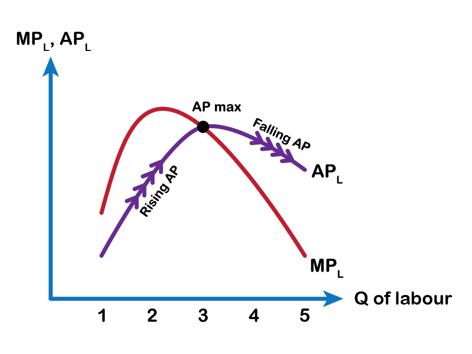
The average product of labour is the total product divided by the quantity of labour. AP=TP/L. What we observe from the third and fourth columns of Fig 7.2 is that, as the marginal product rises, so does the average product, and as the marginal product starts to diminish, the average product starts falling too. As a general rule as long as,
MP > AP, AP rises
MP < AP, AP falls
MP = AP, AP is maximum (maximum productivity of the business)
This relationship between MP and AP is mathematically true. Suppose, 5 friends plan to go for dinner, each carrying $20. In that case, the average amount that each friend is carrying is ($20 × 5 )÷ 5 = $20. Now suppose a sixth friend joins in for dinner who is carrying $25. Then the average rises to approximately $21. So the amount carried by the sixth friend is like the marginal product in our example, which is greater than the average product of $20, and that pulls up the average to about $21. Conversely, if the sixth friend carries $16, then the average changes to $19. Therefore, we find when the marginal ($16) falls below the average ($20), that pulls the average product down ($19). And when the sixth friend carries the same amount of $20 as the five others, the marginal and average both remain the same at $20.
The graph below shows the MP and the AP curves.

Attribution
"7.1 Building Producer Theory" in Principles of Microeconomics by Dr. Emma Hutchinson, University of Victoria is licensed under a Creative Commons Attribution 4.0 International License, except where otherwise noted.
"7.1 Explicit and Implicit Costs, and Accounting and Economic Profits" in Principles of Economics 2e by OpenStax is licensed under Creative Commons Attribution 4.0 International License.
"Module 6: Firms and their Production Decisions" in Intermediate Microeconomics by Patrick M. Emerson is licensed under a Creative Commons Attribution-NonCommercial-ShareAlike 4.0 International License, except where otherwise noted.

