4.2 Supply and Producer Surplus
When economists talk about supply, they mean the amount of some good or service a producer is willing to supply at each price. The supply curve shows the quantity that firms are willing to supply at each price. Price is what the producer receives for selling one unit of a good or service and willingness to supply depends on the marginal cost of producing each unit. A producer will be willing to supply a quantity as long as the price is at least equal to the marginal cost of production.
Example

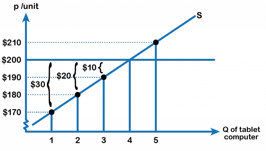
Consider a firm that produces tablet computers. Suppose the price received from selling a computer is $200. Refer to Fig 4.5, the marginal cost of producing the first tablet is $170, the same for the second and third tablets are $180 and $190 respectively. The marginal cost of producing the fourth tablet is $200 and for the fifth tablet is $210. Producer surplus is the difference between the price received from the sale of a good minus the cost of producing that unit. Therefore, the producer surplus from the first, second and third tablets are respectively, $30, $20 and $10. The producer can still manage to produce the fourth tablet, even though the surplus gets to zero because the price is still able to cover the marginal cost of production. However, the producer is unwilling to supply the fifth tablet, as the marginal cost ($210) exceeds the price ($200).
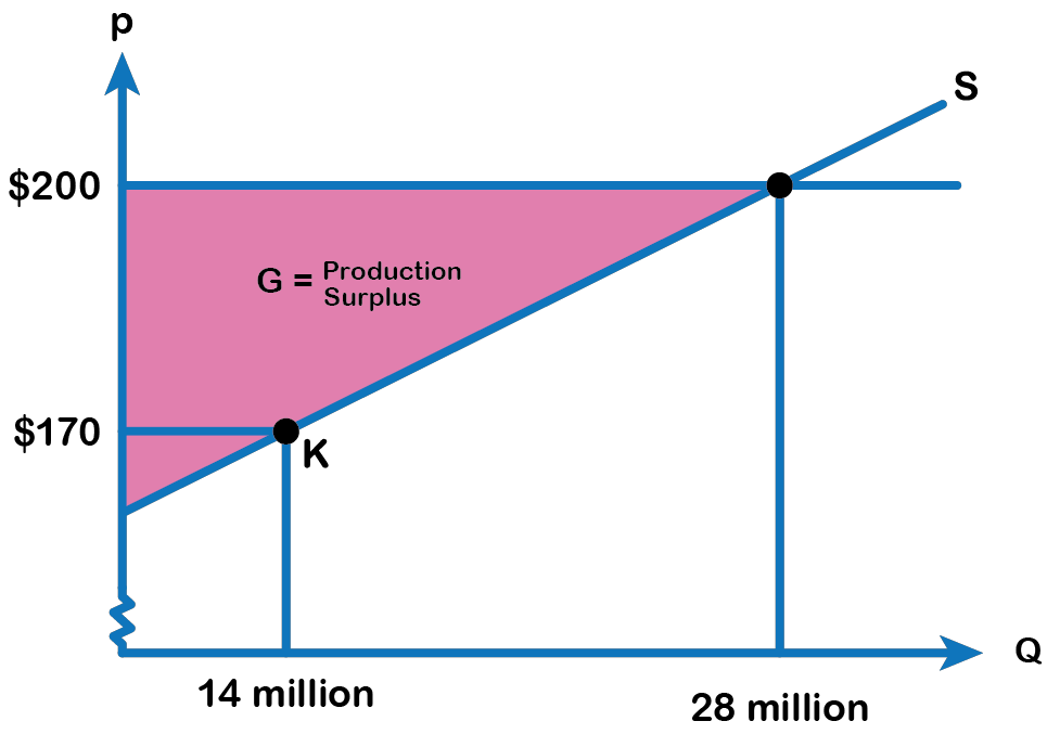
Consider the supply curve for tablet computers in Fig 4.5 below. The price received from the sale of a computer is $200 and the quantity supplied is 28 million. Each point on the supply curve shows the quantity the firm is willing to supply and the willingness depends on the marginal cost of production. The firm would be willing to supply a quantity as long as the price is just enough to cover or exceed the marginal cost of production.

For example, point (K) in Fig 4.6 illustrates that, at $170, firms would still have been willing to supply a quantity of 14 million. Those producers who would have been willing to supply the tablets at $170, but who were instead able to charge a price of $200, clearly received an extra benefit beyond what they required in order to supply the product.
Definition: Producer Surplus
The amount that a seller is paid for a good minus the seller’s actual cost is called producer surplus. In Figure 4.6, producer surplus is the area labelled G—that is, the area between the market price and the segment of the supply curve below the price.
The value of Producer surplus is calculated as the Area of the triangle represented by G.
Producer Surplus = (base × height) ÷ 2
Total Surplus

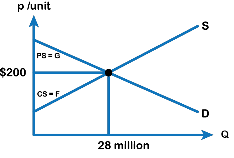
The sum of consumer surplus and producer surplus is social surplus, also referred to as economic surplus or total surplus. In Fig 4.7, we show social surplus as the area F + G. Social surplus is larger at equilibrium quantity and price than it would be at any other quantity. This demonstrates the economic efficiency of the market equilibrium where the marginal benefit from a good just equals the marginal cost of producing it. At the efficient level of output which is also called the competitive equilibrium, it is impossible to produce greater consumer surplus without reducing producer surplus, and it is impossible to produce greater producer surplus without reducing consumer surplus.
Attribution
“3.4 Building Supply and Producer Surplus” in Principles of Microeconomics by Dr. Emma Hutchinson, University of Victoria is licensed under a Creative Commons Attribution 4.0 International License, except where otherwise noted.
“3.1 Demand, Supply, and Equilibrium in Markets for Goods and Services” in Principles of Economics 2e by OpenStax is licensed under Creative Commons Attribution 4.0 International License.

