4.10 – Demand and Supply at Work in Labour Markets
Learning Objectives
- Predict shifts in the demand and supply curves of the labour market
- Explain the impact of new technology on the demand and supply curves of the labour market
- Explain price floors in the labour market such as minimum wage or a living wage
Markets for labour have demand and supply curves, just like markets for goods. The law of demand applies in labour markets this way: A higher salary or wage—that is, a higher price in the labour market—leads to a decrease in the quantity of labour demanded by employers, while a lower salary or wage leads to an increase in the quantity of labour demanded. The law of supply functions in labour markets, too: A higher price for labour leads to a higher quantity of labour supplied; a lower price leads to a lower quantity supplied.
Equilibrium in the Labour Market
In 2015, about 35,000 registered nurses worked in the Minneapolis-St. Paul-Bloomington, Minnesota-Wisconsin metropolitan area, according to the BLS. They worked for a variety of employers: hospitals, doctors’ offices, schools, health clinics, and nursing homes.
Figure 4.10a illustrates how demand and supply determine equilibrium in this labour market. The demand and supply schedules in Table 4.10a list the quantity supplied and quantity demanded of nurses at different salaries.
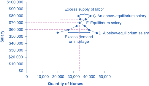
Figure 4.10a (seen above) shows the demand curve (D) of those employers who want to hire nurses intersects with the supply curve (S) of those who are qualified and willing to work as nurses at the equilibrium point (E). The equilibrium salary is $70,000 and the equilibrium quantity is 34,000 nurses. At an above-equilibrium salary of $75,000, quantity supplied increases to 38,000, but the quantity of nurses demanded at the higher pay declines to 33,000. At this above-equilibrium salary, an excess supply or surplus of nurses would exist. At a below-equilibrium salary of $60,000, quantity supplied declines to 27,000, while the quantity demanded at the lower wage increases to 40,000 nurses. At this below-equilibrium salary, excess demand or a shortage exists.
| Annual Salary | Quantity Demanded | Quantity Supplied |
|---|---|---|
| $55,000 | 45,000 | 20,000 |
| $60,000 | 40,000 | 27,000 |
| $65,000 | 37,000 | 31,000 |
| $70,000 | 34,000 | 34,000 |
| $75,000 | 33,000 | 38,000 |
| $80,000 | 32,000 | 41,000 |
The horizontal axis shows the quantity of nurses hired. In this example we measure labour by number of workers, but another common way to measure the quantity of labour is by the number of hours worked. The vertical axis shows the price for nurses’ labour—that is, how much they are paid. In the real world, this “price” would be total labour compensation: salary plus benefits. It is not obvious, but benefits are a significant part (as high as 30 percent) of labour compensation. In this example we measure the price of labour by salary on an annual basis, although in other cases we could measure the price of labour by monthly or weekly pay, or even the wage paid per hour. As the salary for nurses rises, the quantity demanded will fall. Some hospitals and nursing homes may reduce the number of nurses they hire, or they may lay off some of their existing nurses, rather than pay them higher salaries. Employers who face higher nurses’ salaries may also try to replace some nursing functions by investing in physical equipment, like computer monitoring and diagnostic systems to monitor patients, or by using lower-paid health care aides to reduce the number of nurses they need.
As the salary for nurses rises, the quantity supplied will rise. If nurses’ salaries in Minneapolis-St. Paul-Bloomington are higher than in other cities, more nurses will move to Minneapolis-St. Paul-Bloomington to find jobs, more people will be willing to train as nurses, and those currently trained as nurses will be more likely to pursue nursing as a full-time job. In other words, there will be more nurses looking for jobs in the area.
At equilibrium, the quantity supplied and the quantity demanded are equal. Thus, every employer who wants to hire a nurse at this equilibrium wage can find a willing worker, and every nurse who wants to work at this equilibrium salary can find a job. In Figure 4.10a, the supply curve (S) and demand curve (D) intersect at the equilibrium point (E). The equilibrium quantity of nurses in the Minneapolis-St. Paul-Bloomington area is 34,000, and the equilibrium salary is $70,000 per year. This example simplifies the nursing market by focusing on the “average” nurse. In reality, of course, the market for nurses actually comprises many smaller markets, like markets for nurses with varying degrees of experience and credentials. Many markets contain closely related products that differ in quality. For instance, even a simple product like gasoline comes in regular, premium, and super-premium, each with a different price. Even in such cases, discussing the average price of gasoline, like the average salary for nurses, can still be useful because it reflects what is happening in most of the submarkets.
When the price of labour is not at the equilibrium, economic incentives tend to move salaries toward the equilibrium. For example, if salaries for nurses in Minneapolis-St. Paul-Bloomington were above the equilibrium at $75,000 per year, then 38,000 people want to work as nurses, but employers want to hire only 33,000 nurses. At that above-equilibrium salary, excess supply or a surplus results. In a situation of excess supply in the labour market, with many applicants for every job opening, employers will have an incentive to offer lower wages than they otherwise would have. Nurses’ salary will move down toward equilibrium.
In contrast, if the salary is below the equilibrium at, say, $60,000 per year, then a situation of excess demand or a shortage arises. In this case, employers encouraged by the relatively lower wage want to hire 40,000 nurses, but only 27,000 individuals want to work as nurses at that salary in Minneapolis-St. Paul-Bloomington. In response to the shortage, some employers will offer higher pay to attract the nurses. Other employers will have to match the higher pay to keep their own employees. The higher salaries will encourage more nurses to train or work in Minneapolis-St. Paul-Bloomington. Again, price and quantity in the labour market will move toward equilibrium.
Shifts in Labour Demand
The demand curve for labour shows the quantity of labour employers wish to hire at any given salary or wage rate, under the ceteris paribus assumption. A change in the wage or salary will result in a change in the quantity demanded of labour. If the wage rate increases, employers will want to hire fewer employees. The quantity of labour demanded will decrease, and there will be a movement upward along the demand curve. If the wages and salaries decrease, employers are more likely to hire a greater number of workers. The quantity of labour demanded will increase, resulting in a downward movement along the demand curve.
Shifts in the demand curve for labour occur for many reasons. One key reason is that the demand for labour is based on the demand for the good or service that is produced. For example, the more new automobiles consumers demand, the greater the number of workers automakers will need to hire. Therefore the demand for labour is called a “derived demand.” Here are some examples of derived demand for labour:
- The demand for chefs is dependent on the demand for restaurant meals.
- The demand for pharmacists is dependent on the demand for prescription drugs.
- The demand for attorneys is dependent on the demand for legal services.
As the demand for the goods and services increases, the demand for labour will increase, or shift to the right, to meet employers’ production requirements. As the demand for the goods and services decreases, the demand for labour will decrease, or shift to the left. Table 4.10b shows that in addition to the derived demand for labour, demand can also increase or decrease (shift) in response to several factors.
| Factors | Results |
|---|---|
| Demand for Output | When the demand for the good produced (output) increases, both the output price and profitability increase. As a result, producers demand more labour to ramp up production. |
| Education and Training | A well-trained and educated workforce causes an increase in the demand for that labour by employers. Increased levels of productivity within the workforce will cause the demand for labour to shift to the right. If the workforce is not well-trained or educated, employers will not hire from within that labour pool, since they will need to spend a significant amount of time and money training that workforce. Demand for such will shift to the left. |
| Technology | Technology changes can act as either substitutes for or complements to labour. When technology acts as a substitute, it replaces the need for the number of workers an employer needs to hire. For example, word processing decreased the number of typists needed in the workplace. This shifted the demand curve for typists left. An increase in the availability of certain technologies may increase the demand for labour. Technology that acts as a complement to labour will increase the demand for certain types of labour, resulting in a rightward shift of the demand curve. For example, the increased use of word processing and other software has increased the demand for information technology professionals who can resolve software and hardware issues related to a firm’s network. More and better technology will increase demand for skilled workers who know how to use technology to enhance workplace productivity. Those workers who do not adapt to changes in technology will experience a decrease in demand. |
| Number of Companies | An increase in the number of companies producing a given product will increase the demand for labour resulting in a shift to the right. A decrease in the number of companies producing a given product will decrease the demand for labour resulting in a shift to the left. |
| Government Regulations | Complying with government regulations can increase or decrease the demand for labour at any given wage. In the healthcare industry, government rules may require that nurses be hired to carry out certain medical procedures. This will increase the demand for nurses. Less-trained healthcare workers would be prohibited from carrying out these procedures, and the demand for these workers will shift to the left. |
| Price and Availability of Other Inputs | Labour is not the only input into the production process. For example, a salesperson at a call center needs a telephone and a computer terminal to enter data and record sales. If prices of other inputs fall, production will become more profitable and suppliers will demand more labour to increase production. This will cause a rightward shift in the demand curve for labour. The opposite is also true. Higher prices for other inputs lower demand for labour. |
Link It Up
To learn more Georgian College students can access the article Trends and Challenges for Work in the 21st Century [New Tab].
Shifts in Labour Supply
The supply of labour is upward-sloping and adheres to the law of supply: The higher the price, the greater the quantity supplied and the lower the price, the less quantity supplied. The supply curve models the tradeoff between supplying labour into the market or using time in leisure activities at every given price level. The higher the wage, the more labour is willing to work and forego leisure activities. Table 4.10c lists some of the factors that will cause the supply to increase or decrease.
| Factors | Results |
|---|---|
| Number of Workers | An increased number of workers will cause the supply curve to shift to the right. An increased number of workers can be due to several factors, such as immigration, increasing population, an aging population, and changing demographics. Policies that encourage immigration will increase the supply of labour, and vice versa. Population grows when birth rates exceed death rates. This eventually increases supply of labour when the former reach working age. An aging and therefore retiring population will decrease the supply of labour. Another example of changing demographics is more women working outside of the home, which increases the supply of labour. |
| Required Education | The more required education, the lower the supply. There is a lower supply of PhD mathematicians than of high school mathematics teachers; there is a lower supply of cardiologists than of primary care physicians; and there is a lower supply of physicians than of nurses. |
| Government Policies | Government policies can also affect the supply of labour for jobs. Alternatively, the government may support rules that set high qualifications for certain jobs: academic training, certificates or licenses, or experience. When these qualifications are made tougher, the number of qualified workers will decrease at any given wage. On the other hand, the government may also subsidize training or even reduce the required level of qualifications. For example, government might offer subsidies for nursing schools or nursing students. Such provisions would shift the supply curve of nurses to the right. In addition, government policies that change the relative desirability of working versus not working also affect the labour supply. These include unemployment benefits, maternity leave, child care benefits, and welfare policy. For example, child care benefits may increase the labour supply of working mothers. Long term unemployment benefits may discourage job searching for unemployed workers. All these policies must therefore be carefully designed to minimize any negative labour supply effects. |
Technology and Wage Inequality: The Four-Step Process
Economic events can change the equilibrium salary (or wage) and quantity of labour. Consider how the wave of new information technologies, like computer and telecommunications networks, has affected low-skill and high-skill workers in the U.S. economy. From the perspective of employers who demand labour, these new technologies are often a substitute for low-skill labourers like file clerks who used to keep file cabinets full of paper records of transactions. However, the same new technologies are a complement to high-skill workers like managers, who benefit from the technological advances by having the ability to monitor more information, communicate more easily, and juggle a wider array of responsibilities. How will the new technologies affect the wages of high-skill and low-skill workers? For this question, the four-step process of analyzing how shifts in supply or demand affect a market (introduced in Demand and Supply) works in this way:
Step 1. What did the markets for low-skill labour and high-skill labour look like before the arrival of the new technologies? In Figure 4.10b (a) and Figure 4.10b (b), S0 is the original supply curve for labour and D0 is the original demand curve for labour in each market. In each graph, the original point of equilibrium, E0, occurs at the price W0 and the quantity Q0.
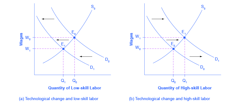
Figure 4.10b Technology and Wages: Applying Demand and Supply (Text Version)
Contains two graphs: Graph A – Technological change and low-skill labour, Graph B – Technological change and high-skill labour.
Graph A: The graph has the vertical axis Wages (W) and Quantity of Low-Skill Labour (Q). The original supply curve (S0) slopes upward from left to right. The original demand Curve (D0) slopes downward from left to right. S0 and D0 intersect at the original equilibrium (E0) at price W0 and quantity Q0 . D0 shifts to the left and now intersects S0 at a new equilibrium (E1) at price W1 and quantity Q1.
Graph B: The graph has the vertical axis Wages (W) and Quantity of High-Skill Labour (Q). The original supply curve (S0) slopes upward from left to right. The original demand Curve (D0) slopes downward from left to right. S0 and D0 intersect at the original equilibrium (E0) at price W0 and quantity Q0 . D1 shifts to the right and now intersects S0 at a new equilibrium (E1) at price W1 and quantity Q1.
Step 2. Does the new technology affect the supply of labour from households or the demand for labour from firms? The technology change described here affects demand for labour by firms that hire workers.
Step 3. Will the new technology increase or decrease demand? Based on the description earlier, as the substitute for low-skill labour becomes available, demand for low-skill labour will shift to the left, from D0 to D1. As the technology complement for high-skill labour becomes cheaper, demand for high-skill labour will shift to the right, from D0 to D1.
Step 4. The new equilibrium for low-skill labour, shown as point E1 with price W1 and quantity Q1, has a lower wage and quantity hired than the original equilibrium, E0. The new equilibrium for high-skill labour, shown as point E1 with price W1 and quantity Q1, has a higher wage and quantity hired than the original equilibrium (E0).
Thus, the demand and supply model predicts that the new computer and communications technologies will raise the pay of high-skill workers but reduce the pay of low-skill workers. From the 1970s to the mid-2000s, the wage gap widened between high-skill and low-skill labour. According to the National Center for Education Statistics, in 1980, for example, a college graduate earned about 30% more than a high school graduate with comparable job experience, but by 2014, a college graduate earned about 66% more than an otherwise comparable high school graduate. Many economists believe that the trend toward greater wage inequality across the U.S. economy is due to improvements in technology.
Link It Up
Learn more about the ten tech skills [New Tab] that have lost relevance in today’s workforce.
Price Floors in the Labour Market: Living Wages and Minimum Wages
In contrast to goods and services markets, price ceilings are rare in labour markets, because rules that prevent people from earning income are not politically popular. There is one exception: boards of trustees or stockholders, as an example, propose limits on the high incomes of top business executives.
The labour market, however, presents some prominent examples of price floors, which are an attempt to increase the wages of low-paid workers. The U.S. government sets a minimum wage, a price floor that makes it illegal for an employer to pay employees less than a certain hourly rate. In mid-2009, the U.S. minimum wage was raised to $7.25 per hour. Local political movements in a number of U.S. cities have pushed for a higher minimum wage, which they call a living wage. Promoters of living wage laws maintain that the minimum wage is too low to ensure a reasonable standard of living. They base this conclusion on the calculation that, if you work 40 hours a week at a minimum wage of $7.25 per hour for 50 weeks a year, your annual income is $14,500, which is less than the official U.S. government definition of what it means for a family to be in poverty. (A family with two adults earning minimum wage and two young children will find it more cost efficient for one parent to provide childcare while the other works for income. Thus the family income would be $14,500, which is significantly lower than the federal poverty line for a family of four, which was $24,250 in 2015.)
Supporters of the living wage argue that full-time workers should be assured a high enough wage so that they can afford the essentials of life: food, clothing, shelter, and healthcare. Since Baltimore passed the first living wage law in 1994, several dozen cities enacted similar laws in the late 1990s and the 2000s. The living wage ordinances do not apply to all employers, but they have specified that all employees of the city or employees of firms that the city hires be paid at least a certain wage that is usually a few dollars per hour above the U.S. minimum wage.
Figure 4.10b illustrates the situation of a city considering a living wage law. For simplicity, we assume that there is no federal minimum wage. The wage appears on the vertical axis, because the wage is the price in the labour market. Before the passage of the living wage law, the equilibrium wage is $10 per hour and the city hires 1,200 workers at this wage. However, a group of concerned citizens persuades the city council to enact a living wage law requiring employers to pay no less than $12 per hour. In response to the higher wage, 1,600 workers look for jobs with the city. At this higher wage, the city, as an employer, is willing to hire only 700 workers. At the price floor, the quantity supplied exceeds the quantity demanded, and a surplus of labour exists in this market. For workers who continue to have a job at a higher salary, life has improved. For those who were willing to work at the old wage rate but lost their jobs with the wage increase, life has not improved. Table 4.10b shows the differences in supply and demand at different wages.
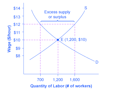
Figure 4.10b A Living Wage: Example of a Price Floor (Text Version)
The graph shows how a price floor results from an excess supply of labour. The vertical axis is Wage ($ per hour) and horizontal axis Quantity of Labour (number of workers). The supply curve (S) slopes upward from left to right and the demand curve (D) slopes downward left to right. S and D intersect at the equilibrium shown at Point E (1,200 workers, $10 per hour). Imposing a wage floor at $12/hour leads to an excess supply of labour. At that wage, the quantity of labour supplied is 1,600 and the quantity of labour demanded is only 700. Table 4.4 Living Wage: Example of a Price Floor details the plotted data.
| Wage | Quantity Labour Demanded | Quantity Labour Supplied |
|---|---|---|
| $8/hr | 1,900 | 500 |
| $9/hr | 1,500 | 900 |
| $10/hr | 1,200 | 1,200 |
| $11/hr | 900 | 1,400 |
| $12/hr | 700 | 1,600 |
| $13/hr | 500 | 1,800 |
| $14/hr | 400 | 1,900 |
The U.S. minimum wage is a price floor that is set either very close to the equilibrium wage or even slightly below it. About 1% of American workers are actually paid the minimum wage. In other words, the vast majority of the U.S. labour force has its wages determined in the labour market, not as a result of the government price floor. However, for workers with low skills and little experience, like those without a high school diploma or teenagers, the minimum wage is quite important. In many cities, the federal minimum wage is apparently below the market price for unskilled labour, because employers offer more than the minimum wage to checkout clerks and other low-skill workers without any government prodding.
Economists have attempted to estimate how much the minimum wage reduces the quantity demanded of low-skill labour. A typical result of such studies is that a 10% increase in the minimum wage would decrease the hiring of unskilled workers by 1 to 2%, which seems a relatively small reduction. In fact, some studies have even found no effect of a higher minimum wage on employment at certain times and places—although these studies are controversial.
Let’s suppose that the minimum wage lies just slightly below the equilibrium wage level. Wages could fluctuate according to market forces above this price floor, but they would not be allowed to move beneath the floor. In this situation, the price floor minimum wage is nonbinding —that is, the price floor is not determining the market outcome. Even if the minimum wage moves just a little higher, it will still have no effect on the quantity of employment in the economy, as long as it remains below the equilibrium wage. Even if the government increases minimum wage by enough so that it rises slightly above the equilibrium wage and becomes binding, there will be only a small excess supply gap between the quantity demanded and quantity supplied.
These insights help to explain why U.S. minimum wage laws have historically had only a small impact on employment. Since the minimum wage has typically been set close to the equilibrium wage for low-skill labour and sometimes even below it, it has not had a large effect in creating an excess supply of labour. However, if the minimum wage increased dramatically—say, if it doubled to match the living wages that some U.S. cities have considered—then its impact on reducing the quantity demanded of employment would be far greater. As of 2017, many U.S. states are set to increase their minimum wage to $15 per hour. We will see what happens. The following Clear It Up feature describes in greater detail some of the arguments for and against changes to minimum wage.
Clear It Up
What’s the harm in raising the minimum wage?
Because of the law of demand, a higher required wage will reduce the amount of low-skill employment either in terms of employees or in terms of work hours. Although there is controversy over the numbers, let’s say for the sake of the argument that a 10% rise in the minimum wage will reduce the employment of low-skill workers by 2%. Does this outcome mean that raising the minimum wage by 10% is bad public policy? Not necessarily.
If 98% of those receiving the minimum wage have a pay increase of 10%, but 2% of those receiving the minimum wage lose their jobs, are the gains for society as a whole greater than the losses? The answer is not clear, because job losses, even for a small group, may cause more pain than modest income gains for others. For one thing, we need to consider which minimum wage workers are losing their jobs. If the 2% of minimum wage workers who lose their jobs are struggling to support families, that is one thing. If those who lose their job are high school students picking up spending money over summer vacation, that is something else.
Another complexity is that many minimum wage workers do not work full-time for an entire year. Imagine a minimum wage worker who holds different part-time jobs for a few months at a time, with bouts of unemployment in between. The worker in this situation receives the 10% raise in the minimum wage when working, but also ends up working 2% fewer hours during the year because the higher minimum wage reduces how much employers want people to work. Overall, this worker’s income would rise because the 10% pay raise would more than offset the 2% fewer hours worked.
Of course, these arguments do not prove that raising the minimum wage is necessarily a good idea either. There may well be other, better public policy options for helping low-wage workers. The lesson from this maze of minimum wage arguments is that complex social problems rarely have simple answers. Even those who agree on how a proposed economic policy affects quantity demanded and quantity supplied may still disagree on whether the policy is a good idea.
Key Concepts and Summary
In the labor market, households are on the supply side of the market and firms are on the demand side. In the market for financial capital, households and firms can be on either side of the market: they are suppliers of financial capital when they save or make financial investments, and demanders of financial capital when they borrow or receive financial investments.
In the demand and supply analysis of labor markets, we can measure the price by the annual salary or hourly wage received. We can measure the quantity of labor various ways, like number of workers or the number of hours worked.
Factors that can shift the demand curve for labor include: a change in the quantity demanded of the product that the labor produces; a change in the production process that uses more or less labor; and a change in government policy that affects the quantity of labor that firms wish to hire at a given wage. Demand can also increase or decrease (shift) in response to: workers’ level of education and training, technology, the number of companies, and availability and price of other inputs.
The main factors that can shift the supply curve for labor are: how desirable a job appears to workers relative to the alternatives, government policy that either restricts or encourages the quantity of workers trained for the job, the number of workers in the economy, and required education.
Attribution
Except where otherise noted, this chapter is adapted from “Demand and Supply at Work in Labor Markets” and “Key Concepts and Summary” In Principles of Microeconomics 2e (Open Stax) by Steven A. Greenlaw & David Shapiro licensed under CC BY 4.0./ Adaptations include addition of glossary terms “Key Terms” In Principles of Microeconomics 2e (Open Stax) by Steven A. Greenlaw & David Shapiro, licensed under CC BY 4.0.
Access for free at Principles of Microeconomics 2e
Original Source References
American Community Survey. 2012. “School Enrollment and Work Status: 2011.” Accessed April 13, 2015. http://www.census.gov/prod/2013pubs/acsbr11-14.pdf.
National Center for Educational Statistics. “Digest of Education Statistics.” (2008 and 2010). Accessed December 11, 2013. nces.ed.gov.
CreditCards.com. 2013. http://www.creditcards.com/credit-card-news/credit-card-industry-facts-personal-debt-statistics-1276.php.
Media Attributions
- 6cf6cd494839cbc9057952a16cae285b96ab03b7 © Steven A. Greenlaw & David Shapiro (OpenStax) is licensed under a CC BY (Attribution) license
- 9ab76f6626367880e8223a824826f5f1716860cc © Steven A. Greenlaw & David Shapiro (OpenStax) is licensed under a CC BY (Attribution) license
- ea6e018685cadfc3b2f5a02489421623286bcdab © Steven A. Greenlaw & David Shapiro (OpenStax) is licensed under a CC BY (Attribution) license
a price floor that makes it illegal for an employer to pay employees less than a certain hourly rate
