5.4 – Polar Cases of Elasticity and Constant Elasticity

There are two extreme cases of elasticity: when elasticity equals zero and when it is infinite. A third case is that of constant unitary elasticity. We will describe each case.
Infinite elasticity or perfect elasticity refers to the extreme case where either the quantity demanded (Qd) or supplied (Qs) changes by an infinite amount in response to any change in price at all. In both cases, the supply and the demand curve are horizontal as Figure 5.4a shows. While perfectly elastic supply curves are for the most part unrealistic, goods with readily available inputs and whose production can easily expand will feature highly elastic supply curves. Examples include pizza, bread, books, and pencils. Similarly, perfectly elastic demand is an extreme example. However, luxury goods, items that take a large share of individuals’ income, and goods with many substitutes are likely to have highly elastic demand curves. Examples of such goods are Caribbean cruises and sports vehicles.

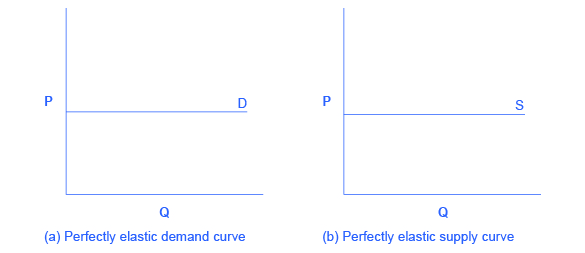
In Figure 5.4a Infinite Elasticity the horizontal lines show that an infinite quantity will be demanded or supplied at a specific price. This illustrates the cases of a perfectly (or infinitely) elastic demand curve and supply curve. The quantity supplied or demanded is extremely responsive to price changes, moving from zero for prices close to P to infinite when prices reach P.
Zero elasticity or perfect inelasticity, as Figure 5.4b depicts, refers to the extreme case in which a percentage change in price, no matter how large, results in zero change in quantity. While a perfectly inelastic supply is an extreme example, goods with limited supply of inputs are likely to feature highly inelastic supply curves. Examples include diamond rings or housing in prime locations such as apartments facing Central Park in New York City. Similarly, while perfectly inelastic demand is an extreme case, necessities with no close substitutes are likely to have highly inelastic demand curves. This is the case of life-saving drugs and gasoline.

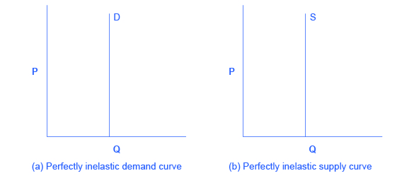
In Figure 5.4b Zero Elasticity the vertical supply curve and vertical demand curve show that there will be zero percentage change in quantity (a) demanded or (b) supplied, regardless of the price.

Constant unitary elasticity, in either a supply or demand curve, occurs when a price change of one percent results in a quantity change of one percent. Figure 5.4c shows a demand curve with constant unit elasticity. Using the midpoint method, you can calculate that between points A and B on the demand curve, the price changes by 66.7% and quantity demanded also changes by 66.7%. Hence, the elasticity equals 1. Between points B and C, price again changes by 66.7% as does quantity, while between points C and D the corresponding percentage changes are again 66.7% for both price and quantity. In each case, then, the percentage change in price equals the percentage change in quantity, and consequently elasticity equals 1. Notice that in absolute value, the declines in price, as you step down the demand curve, are not identical. Instead, the price falls by $8.00 from A to B, by a smaller amount of $4.00 from B to C, and by a still smaller amount of $2.00 from C to D. As a result, a demand curve with constant unitary elasticity moves from a steeper slope on the left and a flatter slope on the right—and a curved shape overall.

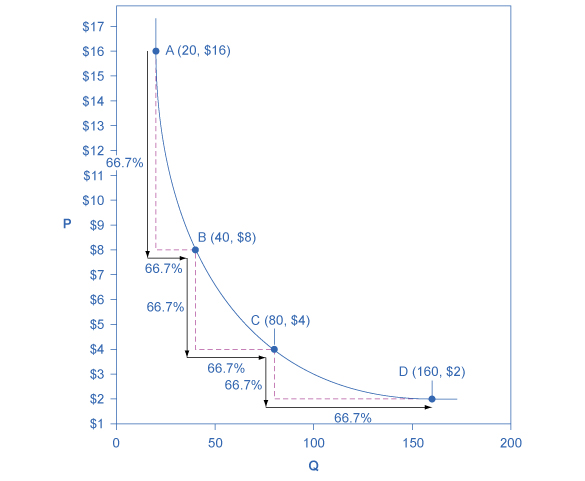
Figure 5.4c. A Constant Unitary Elasticity Demand Curve (Text Version)

The vertical axis is Price (P) in dollars and the horizontal axis Quantity (Q).  The demand curve sloped concave curve downward from left to right and Points A, B, C and D occur along it.  The price and quantity demanded change by an identical percentage amount (66.7%) between each pair of points on the demand curve.

Table 5.4a. A Constant Unitary Elasticity Demand Curve

Point	Point location ( Quantity, Price)
A	20 quantity, 16 dollars
B	40 quantity, 8 dollars
C	80 quantity, 4 dollars
D	160 quantity, 2 dollars

Figure 5.4c A Constant Unitary Elasticity Demand Curve. A demand curve with constant unitary elasticity will be a curved line. Notice how price and quantity demanded change by an identical percentage amount between each pair of points on the demand curve.

Unlike the demand curve with unitary elasticity, the supply curve with unitary elasticity is represented by a straight line, and that line goes through the origin. In each pair of points on the supply curve there is an equal difference in quantity of 30. However, in percentage value, using the midpoint method, the steps are decreasing as one moves from left to right, from 28.6% to 22.2% to 18.2%, because the quantity points in each percentage calculation are getting increasingly larger, which expands the denominator in the elasticity calculation of the percentage change in quantity.

Consider the price changes moving up the supply curve in Figure 5.4d. From points D to E to F and to G on the supply curve, each step of $1.50 is the same in absolute value. However, if we measure the price changes in percentage change terms, using the midpoint method, they are also decreasing, from 28.6% to 22.2% to 18.2%, because the original price points in each percentage calculation are getting increasingly larger in value, increasing the denominator in the calculation of the percentage change in price. Along the constant unitary elasticity supply curve, the percentage quantity increases on the horizontal axis exactly match the percentage price increases on the vertical axis—so this supply curve has a constant unitary elasticity at all points.

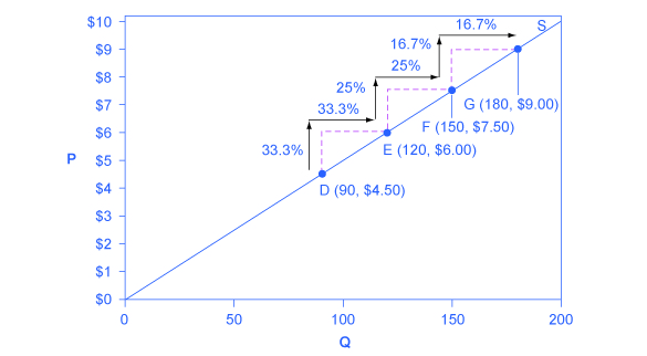
Figure 5.4d. A Constant Unitary Elasticity Supply Curve (Text Version)

A constant unitary elasticity supply curve is a straight line reaching up from the origin. Between each pair of points, the percentage increase in quantity supplied is the same as the percentage increase in price. The vertical axis is Price (P) and the horizontal axis is Quantity (Q). The supply curve (S) slopes upward from left to right. Points D, E, F, and G occur along the supply line is detailed in the table below.

Table 5.4b. A Constant Unitary Elasticity Supply Curve

Point	Point location ( Quantity, Price)
D	90 quantity, 4.50 dollars
E	120 quantity, 6 dollars
F	150 quantity, 7.50 dollars
G	180 quantity, 9 dollars

The percentage value increases in steps between points:

1. Point D to E increases by 33.3%
2. Point E to F increases 25%
3. Point F to G increases 16.7%

Key Concepts and Summary

Infinite or perfect elasticity refers to the extreme case where either the quantity demanded or supplied changes by an infinite amount in response to any change in price at all. Zero elasticity refers to the extreme case in which a percentage change in price, no matter how large, results in zero change in quantity. Constant unitary elasticity in either a supply or demand curve refers to a situation where a price change of one percent results in a quantity change of one percent.

Attribution

Except where otherwise noted, this chapter is adapted from “Polar Cases of Elasticity and Constant Elasticity” and “Key Concepts and Summary” In Principles of Microeconomics 2e (OpenStx) by Steven A. Greenlaw & David Shapiro, licensed under CC BY 4.0./Adaptations include addition of chapter key concepts and summary.

Access for free at Principles of Microeconomics 2e

Original Source Chapter References

Abkowitz, A. “How Netflix got started: Netflix founder and CEO Reed Hastings tells Fortune how he got the idea for the DVD-by-mail service that now has more than eight million customers.” CNN Money. Last Modified January 28, 2009. http://archive.fortune.com/2009/01/27/news/newsmakers/hastings_netflix.fortune/index.htm.

Associated Press (a). ”Analyst: Coinstar gains from Netflix pricing moves.” Boston Globe Media Partners, LLC. Accessed June 24, 2013. http://www.boston.com/business/articles/2011/10/12/analyst_coinstar_gains_from_netflix_pricing_moves/.

Associated Press (b). “Netflix loses 800,000 US subscribers in tough 3Q.” ABC Inc. Accessed June 24, 2013. http://abclocal.go.com/wpvi/story?section=news/business&id=8403368

Baumgardner, James. 2014. “Presentation on Raising the Excise Tax on Cigarettes: Effects on Health and the Federal Budget.” Congressional Budget Office. Accessed March 27, 2015. http://www.cbo.gov/sites/default/files/45214-ICA_Presentation.pdf.

Funding Universe. 2015. “Netflix, Inc. History.” Accessed March 11, 2015. http://www.fundinguniverse.com/company-histories/netflix-inc-history/.

Laporte, Nicole. “A tale of two Netflix.” Fast Company 177 (July 2013) 31-32. Accessed December 3 2013. http://www.fastcompany-digital.com/fastcompany/20130708?pg=33#pg33

Liedtke, Michael, The Associated Press. “Investors bash Netflix stock after slower growth forecast – fee hikes expected to take toll on subscribers most likely to shun costly bundled Net, DVD service.” The Seattle Times. Accessed June 24, 2013 from NewsBank on-line database (Access World News).

Netflix, Inc. 2013. “A Quick Update On Our Streaming Plans And Prices.” Netflix (blog). Accessed March 11, 2015. http://blog.netflix.com/2014/05/a-quick-update-on-our-streaming-plans.html.

Organization for Economic Co-Operation and Development (OECC). n.d. “Average annual hours actually worked per worker.” Accessed March 11, 2015. https://stats.oecd.org/Index.aspx?DataSetCode=ANHRS.

Savitz, Eric. “Netflix Warns DVD Subs Eroding; Q4 View Weak; Losses Ahead; Shrs Plunge.” Forbes.com, 2011. Accessed December 3, 2013. http://www.forbes.com/sites/ericsavitz/2011/10/24/netflix-q3-top-ests-but-shares-hit-by-weak-q4-outlook/.

Statistica.com. 2014. “Coffee Export Volumes Worldwide in November 2014, by Leading Countries (in 60-kilo sacks).” Accessed March 27, 2015. http://www.statista.com/statistics/268135/ranking-of-coffee-exporting-countries/.

Stone, Marcie. “Netflix responds to customers angry with price hike; Netflix stock falls 9%.” News & Politics Examiner, 2011. Clarity Digital Group. Accessed June 24, 2013. http://www.examiner.com/article/netflix-responds-to-customers-angry-with-price-hike-netflix-stock-falls-9.

Weinman, J. (2012). Die hard, hardly dying. Maclean’s, 125(18), 44.

The World Bank Group. 2015. “Gross Savings (% of GDP).” Accessed March 11, 2015. http://data.worldbank.org/indicator/NY.GNS.ICTR.ZS.

Yahoo Finance. Retrieved from http://finance.yahoo.com/q?s=NFLX