11.2 – Productivity and education

Human capital is the result of past investment that raises future incomes. A critical choice for individuals is to decide upon exactly how much additional human capital to accumulate. The cost of investing in another year of school is the direct cost, such as school fees, plus the indirect, or opportunity, cost, which can be measured by the foregone earnings during that extra year. The benefit of the additional investment is that the future flow of earnings is augmented. Consequently, wage differentials should reflect different degrees of education-dependent productivity.

Age-earnings profiles

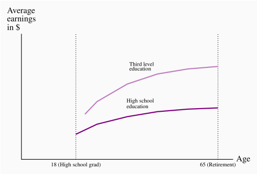
Figure 11.2a illustrates two typical age-earnings profiles for individuals with different levels of education. These profiles define the typical pattern of earnings over time, and are usually derived by examining averages across individuals in surveys. Two aspects are clear: People with more education not only earn more, but the spread tends to grow with time. Less educated, healthy young individuals who work hard may earn a living wage but, unlike their more educated counterparts, they cannot look forward to a wage that rises substantially over time. More highly-educated individuals go into jobs and occupations that take a longer time to master: Lawyers, doctors and most professionals not only undertake more schooling than truck drivers, they also spend many years learning on the job, building up a clientele and accumulating expertise.

Age-earnings profiles define the pattern of earnings over time for individuals with different characteristics.

The education premium

Individuals with different education levels earn different wages. The education premium is the difference in earnings between the more and less highly educated. Quantitatively, Professors Kelly Foley and David Green have recently proposed that the completion of a college or trade certification adds about 15% to one’s income, relative to an individual who has completed high school. A Bachelor’s degree brings a premium of 20-25%, and a graduate degree several percentage points more1. The failure to complete high school penalizes individuals to the extent of about 10%. These are average numbers, and they vary depending upon the province of residence, time period and gender. Nonetheless the findings underline that more human capital is associated with higher earnings. The earnings premium depends upon both the supply and demand of high HK individuals. Ceteris paribus, if high-skill workers are heavily in demand by employers, then the premium should be greater than if lower-skill workers are more in demand.

Education premium: the difference in earnings between the more and less highly educated.

The distribution of earnings has become more unequal in Canada and the US in recent decades, and one reason that has been proposed for this development is that the modern economy demands more high-skill workers; in particular that technological change has a bigger impact on productivity when combined with high-skill workers than with low-skill workers. Consider Figure 11.2b which contains supply and demand functions with a twist. We imagine that there are two types of labour: One with a high level of human capital, the other with a lower level. The vertical axis measures the wage premium of the high-education group (which can be measured in dollars or percentage terms), and the horizontal axis measures the fraction of the total labour force that is of the high-skill type. D is the relative demand for the high skill workers, in this example for the economy as a whole. There is some degree of substitution between high and low-skill workers in the modern economy. We do not propose that several low-skill workers can perform the work of one neuro-surgeon; but several individual households (low-skill) could complete their income tax submissions in the same time as one skilled tax specialist. In this example there is a degree of substitutability. In a production environment, a high-skill manager, equipped with technology and capital, can perform the tasks of several line workers.

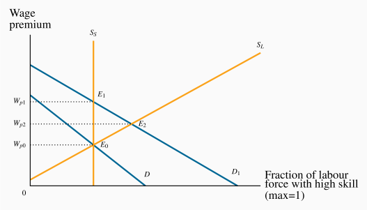
In the short run the make-up of the labour force is fixed, and this is reflected in the vertical supply curve S_s. The equilibrium is at E₀, andW_p⁰ is the premium, or excess, paid to the higher-skill worker over the lower-skill worker. In the long run it is possible for the economy to change the composition of its labour supply: If the wage premium increases, more individuals will find it profitable to train as high-skill workers. That is to say, the fraction of the total that is high-skill increases. It follows that the long-run supply curve slopes upwards.

So what happens when there is an increase in the demand for high-skill workers relative to low-skill workers? The demand curve shifts upward to D₁ , and the new equilibrium is at E₁. The supply mix is fixed in the short run, so there is an increase in the wage premium. But over time, some individuals who might have been just indifferent between educating themselves more and going into the workplace with lower skill levels now find it worthwhile to pursue further education. Their higher anticipated returns to the additional human capital they invest in now exceed the additional costs of more schooling, whereas before the premium increase these additional costs and benefits were in balance. In Figure 13.2 the new short-run equilibrium at has a corresponding wage premium of W_p¹ . In the long run, after additional supply has reached the market, the increased premium is moderated to W_p² at the equilibrium E₂ .

This figure displays what many economists believe has happened in North America in recent decades: The demand for high HK individuals has increased, and the additional supply has not been as great. Consequently the wage premium for the high-skill workers has increased. As we describe later in this chapter, that is not the only perspective on what has happened.

Are students credit-constrained or culture-constrained?

The foregoing analysis assumes that students and potential students make rational decisions on the costs and benefits of further education and act accordingly. It also assumes implicitly that individuals can borrow the funds necessary to build their human capital: If the additional returns to further education are worthwhile, individuals should borrow the money to make the investment, just as entrepreneurs do with physical capital.

However, there is a key difference in the credit markets. If an entrepreneur fails in her business venture the lender will have a claim on the physical capital. But a bank cannot repossess a human being who drops out of school without having accumulated the intended human capital. Accordingly, the traditional lending institutions are frequently reluctant to lend the amount that students might like to borrow—students are credit constrained. The sons and daughters of affluent families therefore find it easier to attend university, because they are more likely to have a supply of funds domestically. Governments customarily step into the breach and supply loans and bursaries to students who have limited resources. While funding frequently presents an obstacle to attending a third-level institution, a stronger determinant of attendance is the education of the parents, as detailed in Application Box 13.1.

Application Box 13.1 Parental education and university attendance in Canada

The biggest single determinant of university attendance in the modern era is parental education. A recent study* of who goes to university examined the level of parental education of young people ‘in transition’ – at the end of their high school – for the years 1991 and 2000.

For the year 2000 they found that, if a parent had not completed high school, there was just a 12% chance that their son would attend university and an 18% chance that a daughter would attend. In contrast, for parents who themselves had completed a university degree, the probability that a son would also attend university was 53% and for a daughter 62%. Hence, the probability of a child attending university was roughly four times higher if the parent came from the top educational category rather than the bottom category! Furthermore the authors found that this probability gap opened wider between 1991 and 2000.

In the United States, Professor Sear Reardon of Stanford University has followed the performance of children from low-income households and compared their achievement with children from high-income households. He has found that the achievement gap between these groups of children has increased substantially over the last three decades. The reason for this growing separation is not because children from low-income households are performing worse in school, it is because high-income parents invest much more of their time and resources in educating their children, both formally in the school environment, and also in extra-school activities.

*Finnie, R., C. Laporte and E. Lascelles. “Family Background and Access to Post-Secondary Education: What Happened in the Nineties?” Statistics Canada Research Paper, Catalogue number 11F0019MIE-226, 2004

Reardon, Sean, “The Great Divide”, New York Times, April 8, 2015.

Attribution

Except where otherwise noted, this chapter is adapted from “Productivity and education” In Principles of Microeconomics (Curtis and Irvine) (LibreText) by Douglas Curtis and Ian Irvine, an adaptation of Principles of Microeconomics, licensed under CC BY-NC-SA 4.0 International.