9.4 – The Poverty Trap
Learning Objectives
- Explain the poverty trap, noting how government programs impact it
- Identify potential issues in government programs that seek to reduce poverty
- Calculate a budget constraint line that represents the poverty trap
Can you give people too much help, or the wrong kind of help? When people are provided with food, shelter, healthcare, income, and other necessities, assistance may reduce their incentive to work. Consider a program to fight poverty that works in this reasonable-sounding manner: the government provides assistance to the poor, but as the poor earn income to support themselves, the government reduces the level of assistance it provides. With such a program, every time a poor person earns $100, the person loses $100 in government support. As a result, the person experiences no net gain for working. Economists call this problem the poverty trap.
Consider the situation a single-parent family faces. Figure 9.4a illustrates a single mother (earning $8 an hour) with two children. First, consider the labour-leisure budget constraint that this family faces in a situation without government assistance. On the horizontal axis is hours of leisure (or time spent with family responsibilities) increasing in quantity from right to left. Also on the horizontal axis is the number of hours at paid work, going from zero hours on the right to the maximum of 2,500 hours on the left. On the vertical axis is the amount of income per year rising from low to higher amounts of income. The budget constraint line shows that at zero hours of leisure and 2,500 hours of work, the maximum amount of income is $20,000 ([latex]{\scriptsize\ $8 \times 2,500\ ; \text{hours}}[/latex]). At the other extreme of the budget constraint line, an individual would work zero hours, earn zero income, but enjoy 2,500 hours of leisure. At point A on the budget constraint line, by working 40 hours a week, 50 weeks a year, the utility-maximizing choice is to work a total of 2,000 hours per year and earn $16,000.
Now suppose that a government antipoverty program guarantees every family with a single mother and two children $18,000 in income. This is represented on the graph by a horizontal line at $18,000. With this program, each time the mother earns $1,000, the government will deduct $1,000 of its support. Table 9.4a shows what will happen at each combination of work and government support.
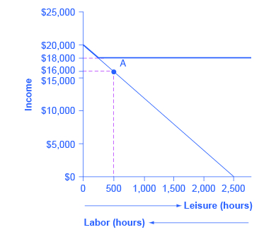
The graph shows a downward sloping line that begins at $20,000 on the y-axis and ends at 2,500 on the x-axis. A horizontal line extends from $18,000 on the y-axis. A dashed plum line extends from $16,000 on the y-axis and intersects with the vertical line extending from 500 on the x-axis at point A. Beneath the x-axis is an arrow pointing to the right indicating leisure (hours) and an arrow pointing to the left indicating labor (hours).
| Amount Worked (hours) | Total Earnings ($) | Government Support ($) | Total Income ($) |
|---|---|---|---|
| 0 | 0 | 18,000 | 18,000 |
| 500 | 4,000 | 14,000 | 18,000 |
| 1,000 | 8,000 | 10,000 | 18,000 |
| 1,500 | 12,000 | 6,000 | 18,000 |
| 2,000 | 16,000 | 2,000 | 18,000 |
| 2,500 | 20,000 | 0 | 20,000 |
The new budget line, with the antipoverty program in place, is the horizontal and heavy line that is flat at $18,000. If the mother does not work at all, she receives $18,000, all from the government. If she works full time, giving up 40 hours per week with her children, she still ends up with $18,000 at the end of the year. Only if she works 2,300 hours in the year—which is an average of 44 hours per week for 50 weeks a year—does household income rise to $18,400. Even in this case, all of her year’s work means that household income rises by only $400 over the income she would receive if she did not work at all. She would need to work 50 hours a week to reach $20,000.
The poverty trap is even stronger than this simplified example shows, because a working mother will have extra expenses like clothing, transportation, and child care that a nonworking mother will not face, making the economic gains from working even smaller. Moreover, those who do not work fail to build up job experience and contacts, which makes working in the future even less likely.
To reduce the poverty trap the government could design an antipoverty program so that, instead of reducing government payments by $1 for every $1 earned, the government would reduce payments by some smaller amount instead. Imposing requirements for work as a condition of receiving benefits and setting a time limit on benefits can also reduce the harshness of the poverty trap.
Figure 9.4b has the vertical axis income and a horizontal axis labour hours. Figure 9.4b illustrates a government program that guarantees $18,000 in income, even for those who do not work at all, but then reduces this amount by 50 cents for each $1 earned. The new, higher budget line in Figure 9.4b shows that, with this program, additional hours of work will bring some economic gain. Because of the reduction in government income when an individual works, an individual earning $8.00 will really net only $4.00 per hour. The vertical intercept of this higher budget constraint line is at $28,000 ([latex]{\scriptsize\$18,000 + 2,500 \; \text{hours} \times $4.00 = $28,000}[/latex]). The horizontal intercept is at the point on the graph where $18,000 and 2500 hours of leisure is set. Table 9.4b shows the total income differences with various choices of labour and leisure.
However, this type of program raises other issues. First, even if it does not eliminate the incentive to work by reducing government payments by $1 for every $1 earned, enacting such a program may still reduce the incentive to work. At least some people who would be working 2,000 hours each year without this program might decide to work fewer hours but still end up with more income—that is, their choice on the new budget line would be like S, above and to the right of the original choice P. Of course, others may choose a point like R, which involves the same amount of work as P, or even a point to the left of R that involves more work.
The second major issue is that when the government phases out its support payments more slowly, the antipoverty program costs more money. Still, it may be preferable in the long run to spend more money on a program that retains a greater incentive to work, rather than spending less money on a program that nearly eliminates any gains from working.
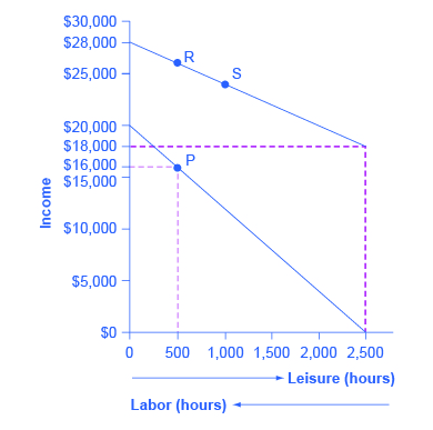
Figure 9.4b Loosening the Poverty Trap: Reducing Government Assistance by 50 Cents for Every $1 Earned
The x-axis is leisure (hours) and y-axis is Income in thousands. The graph shows a downward sloping line that extends from $28,000 on the y-axis to $18,000 on the y-axis (from 0 to 2,500 on the x-axis). Two points R and S appear on the line. Another line starts at (0, $20,000) and ends at (2,500, 0). A dashed plum line extends horizontally from $18,000 on the y-axis and meets with the vertical line extending from 2,500 on the x-axis. Another dashed plum line extends from $16,000 on the y-axis and intersects with the vertical line extending from 500 on the x-axis at point P. Beneath the x-axis is an arrow pointing to the right indicating leisure (hours) and an arrow pointing to the left indicating labour (hours).
| Amount Worked (hours) | Total Earnings ($) | Government Support ($) | Total Income ($) |
|---|---|---|---|
| 0 | 0 | 18,000 | 18,000 |
| 500 | 4,000 | 16,000 | 20,000 |
| 1,000 | 8,000 | 14,000 | 22,000 |
| 1,500 | 12,000 | 12,000 | 24,000 |
| 2,000 | 16,000 | 10,000 | 26,000 |
| 2,500 | 20,000 | 8,000 | 28,000 |
The next module will consider a variety of government support programs focused specifically on the poor, including welfare, SNAP (Supplemental Nutrition Assistance Program), Medicaid, and the earned income tax credit (EITC). Although these programs vary from state to state, it is generally a true statement that in many states from the 1960s into the 1980s, if poor people worked, their level of income barely rose—or did not rise at all—after factoring in the reduction in government support payments. The following Work It Out feature shows how this happens.
Work It Out
Calculating a Budget Constraint Line
Step 1. Determine the amount of the government guaranteed income. In this case, it is $10,000.
Step 2. Plot that guaranteed income as a horizontal line on the budget constraint line.
Step 3. Determine what Jason earns if he has no income and enjoys 2,500 hours of leisure. In this case, he will receive the guaranteed $10,000 (the horizontal intercept).
Step 4. Calculate how much Jason’s salary will be reduced due to the reduction in government income. In Jason’s case, it will be reduced by one half. He will, in effect, net only $4.50 an hour.
Step 5. If Jason works 1,000 hours, at a maximum what income will Jason receive? Jason will receive $10,000 in government assistance. He will net only $4.50 for every hour he chooses to work. If he works 1,000 hours at $4.50, his earned income is $4,500 plus the $10,000 in government income. Thus, the total maximum income (the vertical intercept) is [latex]{\scriptsize\$10,000 + $4,500 = $14,500}[/latex].
Key Concepts and Summary
A poverty trap occurs when government-support payments for the poor decline as the poor earn more income. As a result, the poor do not end up with much more income when they work, because the loss of government support largely or completely offsets any income that one earns by working. Phasing out government benefits more slowly, as well as imposing requirements for work as a condition of receiving benefits and a time limit on benefits can reduce the harshness of the poverty trap.
Attribution
Except where otherwise noted, this chapter is adapted from “The Poverty Trap” and “Key Concepts and Summary” In Principles of Economics 2e by Steven A. Greenlaw & David Shapiro, licensed under CC BY 4.0./ Adaptations include the addition of chapter key concepts and summary.
Access for free at Principles of Microeconomics 2e
Original Source Chapter References
Ebeling, Ashlea. 2014. “IRS Announces 2015 Estate And Gift Tax Limits.” Forbes. Accessed March 16, 2015. http://www.forbes.com/sites/ashleaebeling/2014/10/30/irs-announces-2015-estate-and-gift-tax-limits/.
Federal Register: The Daily Journal of the United States Government. “State Median Income Estimates for a Four-Person Household: Notice of the Federal Fiscal Year (FFY) 2013 State Median Income Estimates for Use Under the Low Income Home Energy Assistance Program (LIHEAP).” Last modified March 15, 2012. https://www.federalregister.gov/articles/2012/03/15/2012-6220/state-median-income-estimates-for-a-four-person-household-notice-of-the-federal-fiscal-year-ffy-2013#t-1.
Luhby, Tami. 2014. “Income is on the rise . . . finally!” Accessed April 10, 2015. http://money.cnn.com/2014/08/20/news/economy/median-income/.
Meyer, Ali. 2015. “56,023,000: Record Number of Women Not in Labor Force.” CNSNews.com. Accessed March 16, 2015. http://cnsnews.com/news/article/ali-meyer/56023000-record-number-women-not-labor-force.
Orshansky, Mollie. “Children of the Poor.” Social Security Bulletin. 26 no. 7 (1963): 3–13. http://www.ssa.gov/policy/docs/ssb/v26n7/v26n7p3.pdf.
The World Bank. “Data: Poverty Headcount Ratio at $1.25 a Day (PPP) (% of Population).” http://data.worldbank.org/indicator/SI.POV.DDAY.
U.S. Department of Commerce: United States Census Bureau. “American FactFinder.” http://factfinder2.census.gov/faces/nav/jsf/pages/index.xhtml.
U.S. Department of Commerce: United States Census Bureau. “Current Population Survey (CPS): CPS Table Creator.” http://www.census.gov/cps/data/cpstablecreator.html.
U.S. Department of Commerce: United States Census Bureau. “Income: Table F-6. Regions—Families (All Races) by Median and Mean Income.” http://www.census.gov/hhes/www/income/data/historical/families/.
U.S. Department of Commerce: United States Census Bureau. “Poverty: Poverty Thresholds.” Last modified 2012. http://www.census.gov/hhes/www/poverty/data/threshld/.
U.S. Department of Health & Human Services. 2015. “2015 Poverty Guidelines.” Accessed April 10, 2015. http://www.medicaid.gov/medicaid-chip-program-information/by-topics/eligibility/downloads/2015-federal-poverty-level-charts.pdf.
U.S. Department of Health & Human Services. 2015. “Information on Poverty and Income Statistics: A Summary of 2014 Current Population Survey Data.” Accessed April 13, 2015. http://aspe.hhs.gov/hsp/14/povertyandincomeest/ib_poverty2014.pdf.
Congressional Budget Office. 2015. “The Effects of Potential Cuts in SNAP Spending on Households With Different Amounts of Income.” Accessed April 13, 2015. https://www.cbo.gov/publication/49978.
Falk, Gene. Congressional Research Service. “The Temporary Assistance for Needy Families (TANF) Block Grant: Responses to Frequently Asked Questions.” Last modified October 17, 2013. http://www.fas.org/sgp/crs/misc/RL32760.pdf.
Library of Congress. “Congressional Research Service.” http://www.loc.gov/crsinfo/about/.
Office of Management and Budget. “Fiscal Year 2013 Historical Tables: Budget of the U.S. Government.” http://www.whitehouse.gov/sites/default/files/omb/budget/fy2013/assets/hist.pdf.
Tax Policy Center: Urban Institute and Brookings Institution. “The Tax Policy Briefing Book: Taxation and the Family: What is the Earned Income Tax Credit?” http://www.taxpolicycenter.org/briefing-book/key-elements/family/eitc.cfm.
Frank, Robert H., and Philip J. Cook. The Winner-Take-All Society. New York: Martin Kessler Books at The Free Press, 1995.
Institute of Education Sciences: National Center for Education Statistics. “Fast Facts: Degrees Conferred by Sex and Race.” http://nces.ed.gov/fastfacts/display.asp?id=72.
Nhan, Doris. “Census: More in U.S. Report Nontraditional Households.” National Journal. Last modified May 1, 2012. http://www.nationaljournal.com/thenextamerica/demographics/census-more-in-u-s-report-nontraditional-households-20120430.
U.S. Bureau of Labor Statistics: BLS Reports. “Report 1040: Women in the Labor Force: A Databook.” Last modified March 26, 2013. http://www.bls.gov/cps/wlf-databook-2012.pdf.
U.S. Department of Commerce: United States Census Bureau. “Income: Table H-2. Share of Aggregate Income Received by Each Fifth and Top 5 Percent of Households.” http://www.census.gov/hhes/www/income/data/historical/household/.
United States Census Bureau. 2014. “2013 Highlights.” Accessed April 13, 2015. http://www.census.gov/hhes/www/poverty/about/overview/.
United States Census Bureau. 2014. “Historical Income Tables: Households: Table H-2 Share of Aggregate Income Received by Each Fifth and Top 5% of Income. All Races.” Accessed April 13, 2015. http://www.census.gov/hhes/www/income/data/historical/household/.
Board of Governors of the Federal Reserve System. “Research Resources: Survey of Consumer Finances.” Last modified December 13, 2013. http://www.federalreserve.gov/econresdata/scf/scfindex.htm.
Congressional Budget Office. “The Distribution of Household Income and Federal Taxes, 2008 and 2009.” Last modified July 10, 2012. http://www.cbo.gov/publication/43373.
Huang, Chye-Ching, and Nathaniel Frentz. “Myths and Realities About the Estate Tax.” Center on Budget and Policy Priorities. Last modified August 29, 2013. http://www.cbpp.org/files/estatetaxmyths.pdf.
Media Attributions
- Figure © Steven A. Greenlaw & David Shapiro (OpenStax) is licensed under a CC BY (Attribution) license
- Figure © Steven A. Greenlaw & David Shapiro (OpenStax) is licensed under a CC BY (Attribution) license
The situation of being below a certain level of income one needs for a basic standard of living
Antipoverty programs set up so that government benefits decline substantially as people earn more income—as a result, working provides little financial gain
A method of assisting the working poor through the tax system
